[SATV 0x07] Data Flow Analysis

01 Introduction to Static Analysis

Review some basic concepts in program analysis:

• A program point is the location of an instruction in the program; it is also a value of the PC (Program Counter).
• Invariants are properties that hold at a program point if they hold in any such state for any execution with any input.
• A program analyzer is a program that reasons about programs. Requirements for a perfect program analyzer:
  • Soundness: don’t miss any errors
  • Completeness: don’t raise false alarms
  • Termination: always give an answer

Program analysis is about discovering useful facts about programs. These facts can help us optimize efficiency, ensure correctness, support program understanding and enable refactorings. However, finding them is no easy task. According to Rice’s theorem:

Any non-trivial property¹ of the behavior of programs in a Turing-complete² language is undecidable³!

The answers to non-trivial properties are undecidable. Does that mean there is no way to find answers to these properties?

Although precise answers are undecidable and hard to obtain, approximate answers may be decidable. Approximation must be conservative, i.e., it should err only on “the safe side”. In this lecture, we will focus on decision problems, whose answers are solely “yes” or “no”. (Of course, there are more subtle approximations beyond “yes”/“no”, e.g., memory usage or pointer targets.)

A correct but trivial approximation algorithm may just give the useless answer every time. The engineering challenge is to give the useful answer often enough to fuel the client application, and to do so within reasonable time and space, which is the hard (and fun) part of static analysis!

Static analysis is a technique for examining code before a program is run. It finds potential errors, problems, or optimization opportunities by analyzing the structure and syntax of the code without actually executing it.

Static code analyzers:

• Linters are static analysis tools designed to check code for syntax errors, code style issues, and potential logic errors, such as ESLint, PMD, PyLint…
• Every optimizing compiler and modern JIT use it for optimization.
• Some analysis tools like Astree, Klocwork, and PVS-Studio use it for verification or error detection.

02 Control Flow Graphs

Before actually formulating and implementing an analysis, we need to decide how to represent programs. Two ways to do that are abstract syntax trees (AST) and control flow graphs (CFG). CFG is our focus.

A control flow graph is a directed graph whose nodes correspond to program points, and whose edges represent possible flows of control. A CFG always has two special nodes: entry and exit (think of them as no-op statements).

Let $v$ be a node in a CFG:

• $\mathrm{pred}(v)$ is the set of predecessor nodes
• $\mathrm{succ}(v)$ is the set of successor nodes

An example of a CFG:

A node in a CFG represents a program point, but when the statement is complicated, the node may perform multiple operations, which may hinder analysis. To ensure that each CFG node performs only one operation, it is imperative to normalize a CFG.

Normalization: flatten nested expressions, using fresh variables.

Assuming that we have a statement (a program point):

x=f(y+3)*5;

after normalization, we obtain:

t1=y+3;
t2=f(t1);
x=t2*5;

03 Data Flow Analysis

Basic idea:

• Propagate analysis information along the edges of a control flow graph
• Goal: Compute analysis state at each program point
• For each statement, define how it affects the analysis state
• For loops: Iterate until fix-point reached

3.1 Example: Available Expression Analysis

Available expression analysis is a static code analysis technique used to optimize code in compilers. Its objective is to identify which expressions are “available” at a given point in the code, thus avoiding repeated computation of the same expression and improving the efficiency of code execution.

3.1.1 Available Expressions

In available expression analysis, an “available” expression is one whose result has already been computed at some point in the program, and no operation will change the variables on which the expression depends from that point to the point where the expression is used. Therefore, the result of the expression can be used directly without the need for recalculation.

---

See the below example:

var x = a + b;  
var y = a * b;  
while (y > a + b) {	// a+b is available every time execution reaches this point
    a = a - 1;
    x = a + b;
}

---

3.1.2 Transfer Functions

Transfer functions show how the statement affects the analysis state (available expressions).

There are two transfer functions:

• gen: Available expressions generated by a statement
• kill: Available expressions killed by a statement

---

Example:

int x = a + b;  // stmt1
a = 10;         // stmt2

When the first line of code is executed, the available expression a+b is generated, so $\mathrm{gen}(\text{stmt1})=\{a+b\}$.

When the second line of code is executed, the value of a is changed and thus the value of a+b computed by the first line is no longer effective, i.e. killed, so $\mathrm{kill}(\text{stmt2})=\{a+b\}$.

---

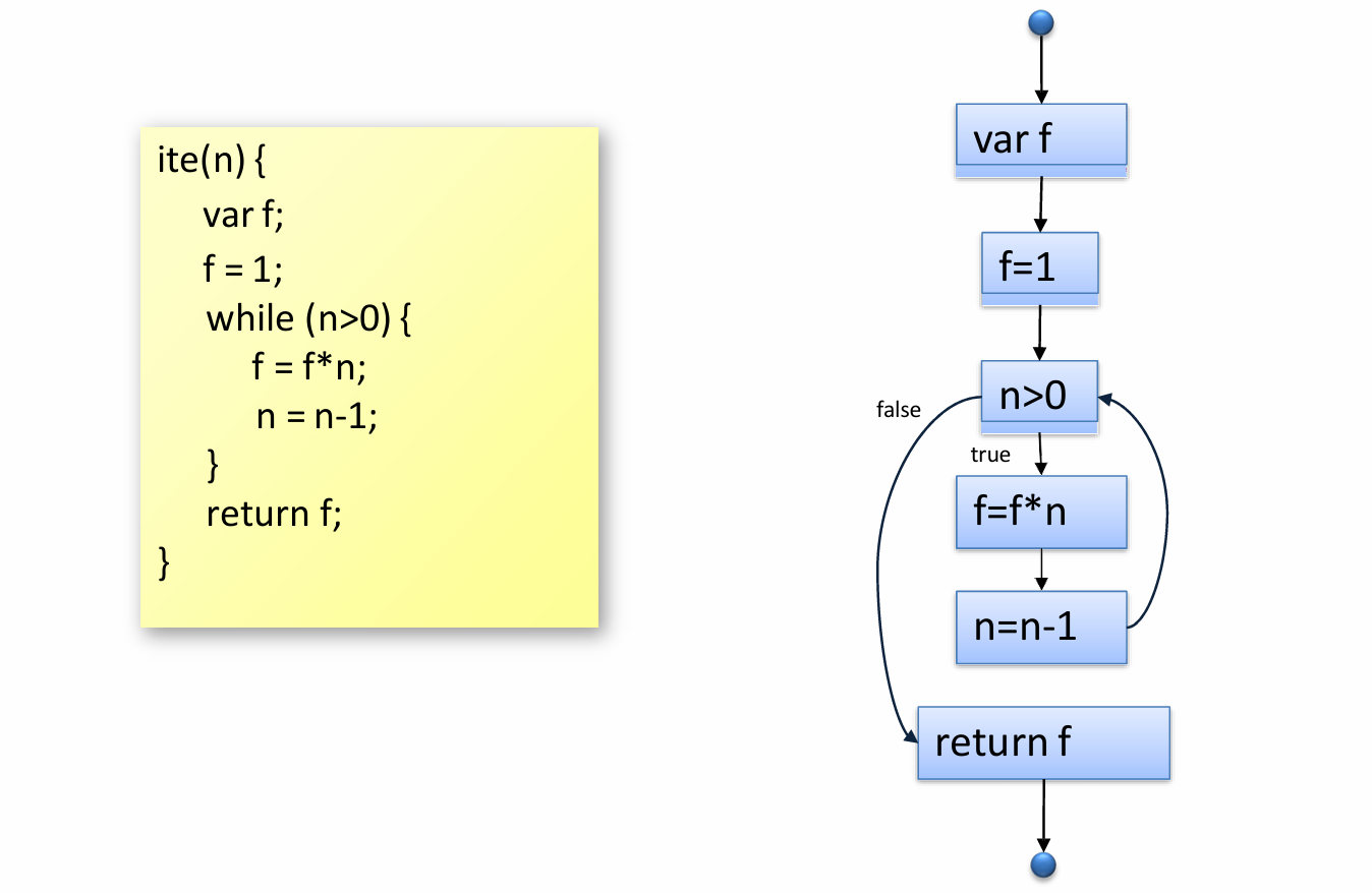
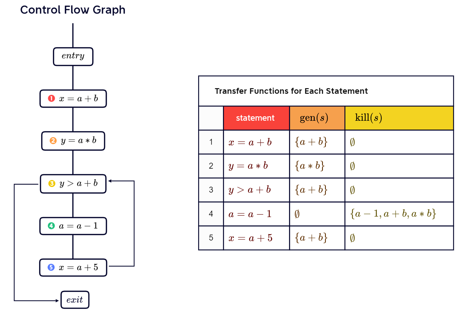
Quiz: Draw a CFG of the following program and give the transfer functions for the first 5 statements.

var x = a + b;  
var y = a * b;  
while (y > a + b) {
    a = a - 1;
    x = a + b;
}

Answer:

---

3.1.3 Propagating Available Expressions

The process of propagating available expressions involves calculating all expressions that are available at each point in the program.

1. Initially, no available expressions
2. Forward analysis: Propagate available expressions in the direction of control flow
3. For each statement $s$, outgoing available expressions are: $\text{incoming available expressions}-\mathrm{kill}(s)+\mathrm{gen}(s)$⁴
4. When control flow splits, propagate available expressions both ways
5. When control flows merge, intersect the incoming available expressions

3.2 Basic Principles

Any data flow analysis is defined by 6 properties:

• Domain (facts)
• Direction
• Transfer function
• Meet operator
• Boundary condition
• Initial values

3.2.1 Domain

Analysis associates some information with every program point. “Information” means elements of a set.

A domain of the analysis points to all possible elements the set may have. E.g., for available expressions analysis, the domain is a set of non-trivial expressions.

3.2.2 Direction

Analysis propagates information along the control flow graph.

Depending on the propagation direction, there are forward and backward analyses. The forward analysis follows normal flow of control, while the backward analysis inverts all edges of the CFG, which reasons about executions in reverse. E.g. available expressions analysis is forward analysis.

3.2.3 Transfer Function

Transfer functions define how a statement affects the propagated information.

For each statement (program point) $s$, let $DF_{entry}(s)$ represent the data flow information at the entry point of the statement $s$. This is the information passed in from the previous code before entering the point, and $DF_{exit}(s)$ the data flow information at the exit of the statement $s$, which is the information that is passed to subsequent code when leaving that point.

Thus we have $DF_{exit}(s)=F(DF_{entry}(s))$ (the function $F$ here represents the operations that $s$ does).

E.g., for available expressions analysis: $AE_{exit}(s)=(AE_{entry}(s)-kill(s))\cup gen(s)$.

3.2.4 Meet Operator

What if two statements $s_{1},s_{2}$ flow to a statement $s$?

• Forward analysis: Execution branches merge
• Backward analysis: Branching point

Meet operator defines how to combine the incoming information:

• Union: $DF_{entry}(s)=DF_{exit}(s_{1})\cup DF_{exit}(s_{2})$
• Intersection: $DF_{entry}(s)=DF_{exit}(s_{1})\cap DF_{exit}(s_{2})$ (e.g. available expressions analysis)

3.2.5 Boundary Condition

What information to start with at the first CFG node?

• Forward analysis: First node is entry node
• Backward analysis: First node is exit node

Common choices:

• Empty set (e.g. available expressions analysis)
• Entire domain

3.2.6 Initial Values

What is the information to start with at intermediate nodes?

Common choices:

• Empty set (e.g. available expressions analysis⁵)
• Entire domain

3.2.7 Defining a Data Flow Analysis

Take available expressions analysis for example:

• Domain: Non-trivial expressions
• Direction: Forward
• Transfer function: $AE_{exit}(s)=(AE_{entry}(s)-kill(s))\cup gen(s)$
• Meet operation: Intersection
• Boundary condition: $AE_{entry}(entryNode)=\emptyset$
• Initial value: $\emptyset$

3.2.8 Classifying Data Flow Analysis

• Forward or backward, or something both
• Whether facts may or must be true:
  • In a may analysis, we care about the facts that may be true at $p$. That is, they are true for some path up to or from $p$, depending on the direction of the analysis.
  • In a must analysis, we care about the facts that must be true at $p$. That is, they are true for every path up to or from $p$.

3.3 More Examples

3.3.1 Reaching Definitions Analysis

Reaching Definitions Analysis is a data flow analysis technique used to determine at each point in a program which variable definitions (assignment operations) reach that point. In short, it helps us understand which variable values are valid at a given point in a program and where those values come from.

Goal: For each program point, compute which assignments may have been made and may not have been overwritten.

This is often useful in various program analyses, e.g., to compute a data flow graph.

---

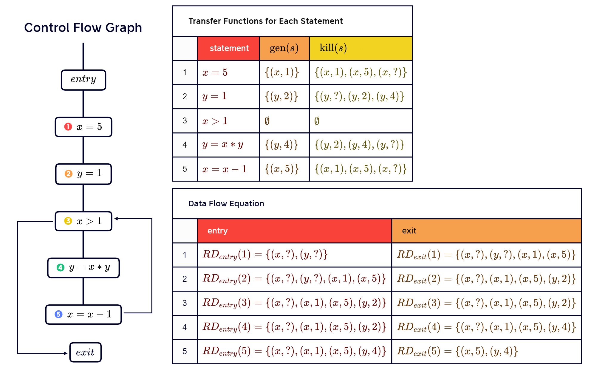
Example:

var x = 5;
var y = 1;
while (x > 1) {
    y = x * y;
    x = x - 1;
}

The definition of x reaches the entry of the statement on line 4.

Three definitions (line 1, 2, 4, 5) reach the entry of the statement on line 4.

---

Define the analysis:

• Domain: Definitions (assignments) in the code
  • Set of pairs $(v, s)$ of variables and statements
  • $(v, s)$ means a definition of $v$ at $s$
• Direction: Forward
• Meet operator: Union
• Transfer function: $RD_{exit}(s)=(RD_{entry}(s)-kill(s))+gen(s)$
  • Function $gen(s)$: If $s$ is an assignment to $v$, $gen(s)=(v,s)$; otherwise, empty set.
  • Function $kill(s)$: If $s$ is an assignment to $v$, $kill(s)=(v,s^{\prime})$ for all $s^{\prime}$ that overwrite $v$; otherwise, empty set.
• Boundary condition: Entry node starts with all variables undefined
  • $RD_{entry}(entryNode)=\{(v,?)|v\in Vars\}$ where $?$ is a special statement for undefined variables
• Initial values: Initially, all nodes have no reaching definitions

---

Continuing the previous example, we draw a CFG and give the data flow chart:

3.3.2 Very Busy Expression Analysis

Very Busy Expression Analysis is a data flow analysis technique used in compiler optimization to identify expressions that are “very busy” at a particular program point. An expression is considered “very busy” if its value is used on all paths from that point to the end of the program. In other words, the expression’s value is always needed and cannot be recomputed without affecting the program’s correctness. This is useful for program optimizations, e.g. hoisting⁶.

Goal: For each program point, find expressions that must be very busy.

---

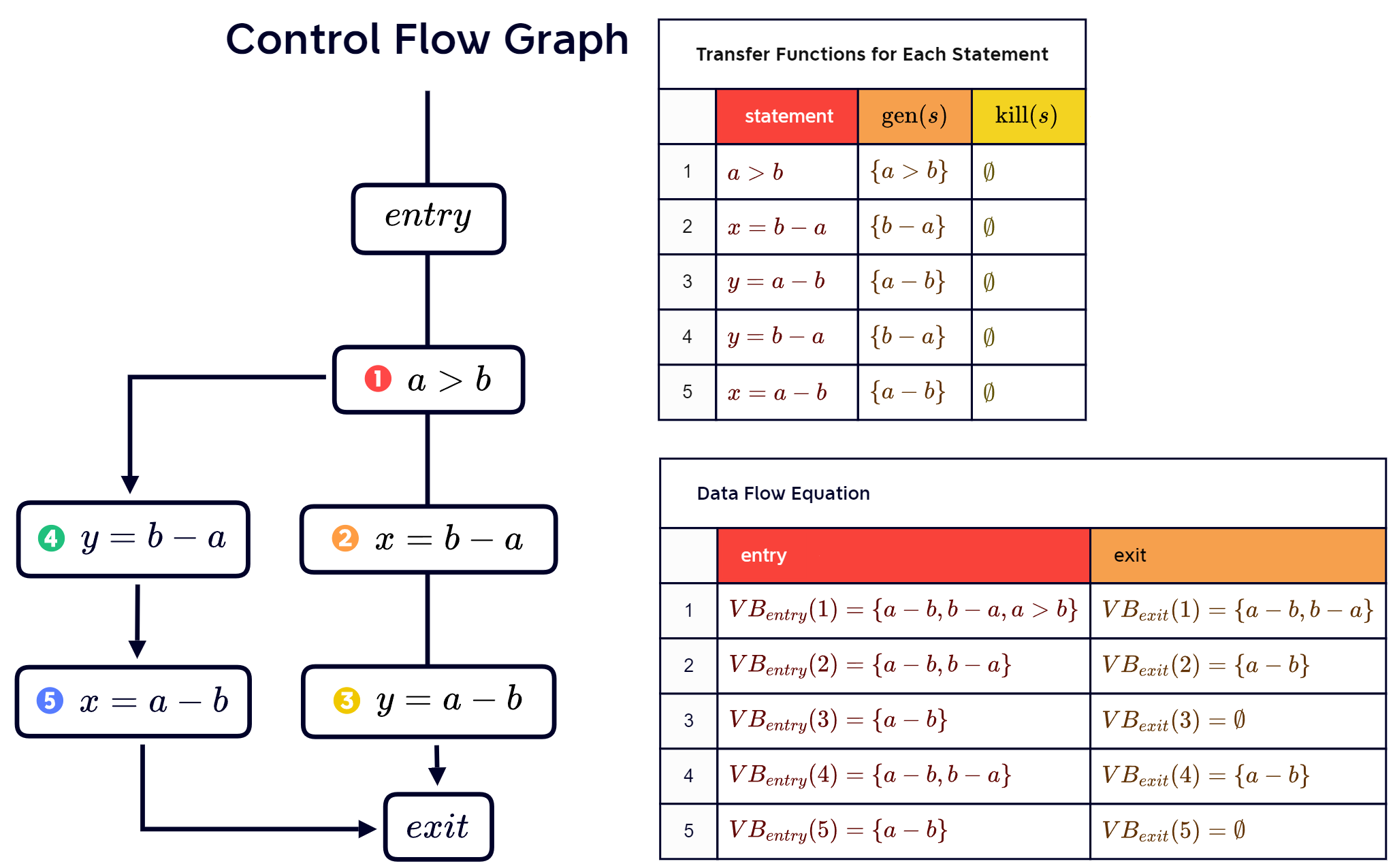
Example:

if (a > b) {  
    x = b - a;
    y = a - b;
} else {
    y = b - a;
    x = a - b;
}

In the above code, we can see that a-b and b-a are very busy.

---

Define the analysis:

• Domain: All non-trivial expressions occurring in the code
• Direction: Backward
• Meet operator: Intersection
• Transfer function: $VB_{entry}(s)=(VB_{exit}(s)-kill(s))\cup gen(s)$
  • Backward analysis: Returns expressions that are very busy expressions at entry of statement
  • Function $gen(s)$: All expressions $e$ that appear in $s$
  • Function $kill(s)$: If $s$ assigns to $x$, all expressions in which $x$ occurs; otherwise, empty set
• Boundary condition: Final node starts with no very busy expressions - $VB_{exit}(finalNode)=\emptyset$
• Initially, all nodes have no very busy expressions

---

Continuing the previous example, we draw a CFG and give the data flow chart:

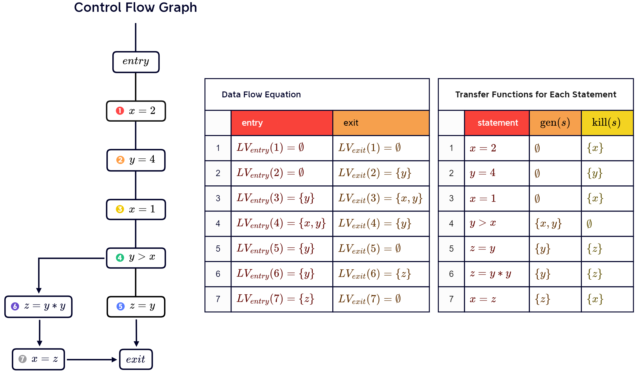
3.3.3 Live Variables Analysis

Live Variables Analysis is a backward data-flow analysis technique used to identify the variables that are live at each point in a program. A variable is considered live at a point if its value might be used in the future along some path of execution from that point. This is useful, e.g., for identifying dead code, such as, bug detection (dead assignments are typically unintended), optimization (remove dead code).

Goal: For each statement, find variables that are may be “live” at the exit from the statement.

“Live”: The variable is used before being redefined.

---

Example:

x = 2;
y = 4;
x = 1;
if (y > x) {  
	z = y;
} else {
    z = y * y;  
    x = z;
}

The x on line 1 is not live because after this statement, it is redefined on line 3.

The y on line 2 and the x on line 3 are live, because they will not be redefined and will be used after.

---

Defining the analysis:

• Domain: All variables occurring in the code
• Direction: Backward
• Meet operator: Union
• Transfer function: $VB_{entry}(s)=(VB_{exit}(s)-kill(s))\cup gen(s)$
• Function $gen(s)$: All variables $v$ that are used in $s$
• Function $kill(s)$: If s assigns to $x$, then it kills $x$
• Boundary condition: Final node starts with no live variables - $LV_{exit}(finalNode)=\emptyset$
• Initially, all nodes have no live variables

---

Continuing the previous example, we draw a CFG and give the data flow chart:

3.4 Solving Data Flow Problems

Transfer functions yield data flow equations for each statement. How to solve these equations? A naive algorithm to solve the problem is Round-robin algorithm, the one we usually use when hand-calculating. We will give the procedure of it and later introduce a more efficient algorithm - work list algorithm.

3.4.1 Round-robin, iterative algorithm

This a naive algorithm for solving data flow equations. The procedure of the algorithm:

1. For each statement $s$, initialize the entry and exit set of $s$.

2. While sets are still changing, for each $s$:

   • update entry set of $s$ by applying meet operator to exit sets of incoming statements

   • compute exit set of $a$ based on its entry set

3.4.2 Work list algorithm

Define a work list $W$ containing all statements that need to be processed. The procedure of the algorithm:

1. For each statement $s$: Initialize the entry and exit set.
2. Initialize $W$ with the initial node.
3. While $W$ not empty:
   • Remove a statement $s$ from $W$ (can be arbitrary)
   • Update the entry set of $s$ by applying meet operator to exit sets of incoming statements
   • Compute the exit set of $s$ based on its entry set
   • If the exit set has changed (or the statement visited for the first time): Add successors of $s$ to $W$

Will the work list algorithm always terminate? In principle, it may run forever. Thus, we need to impose constraints to ensure termination, such as:

• Domain of analysis: Partial order with finite height
• Transfer function and meet operator: Monotonic w.r.t. partial order

3.5 Inter-procedural Analysis

The data flow analysis considered so far is only intra-procedural, which means it reasons about a function in isolation. Inter-procedural analysis reasons about multiple functions.

Inter-procedural control flow:

• One control flow graph per function
• Connect call sites to entry node of callee
• Connect exit node back to call site

---

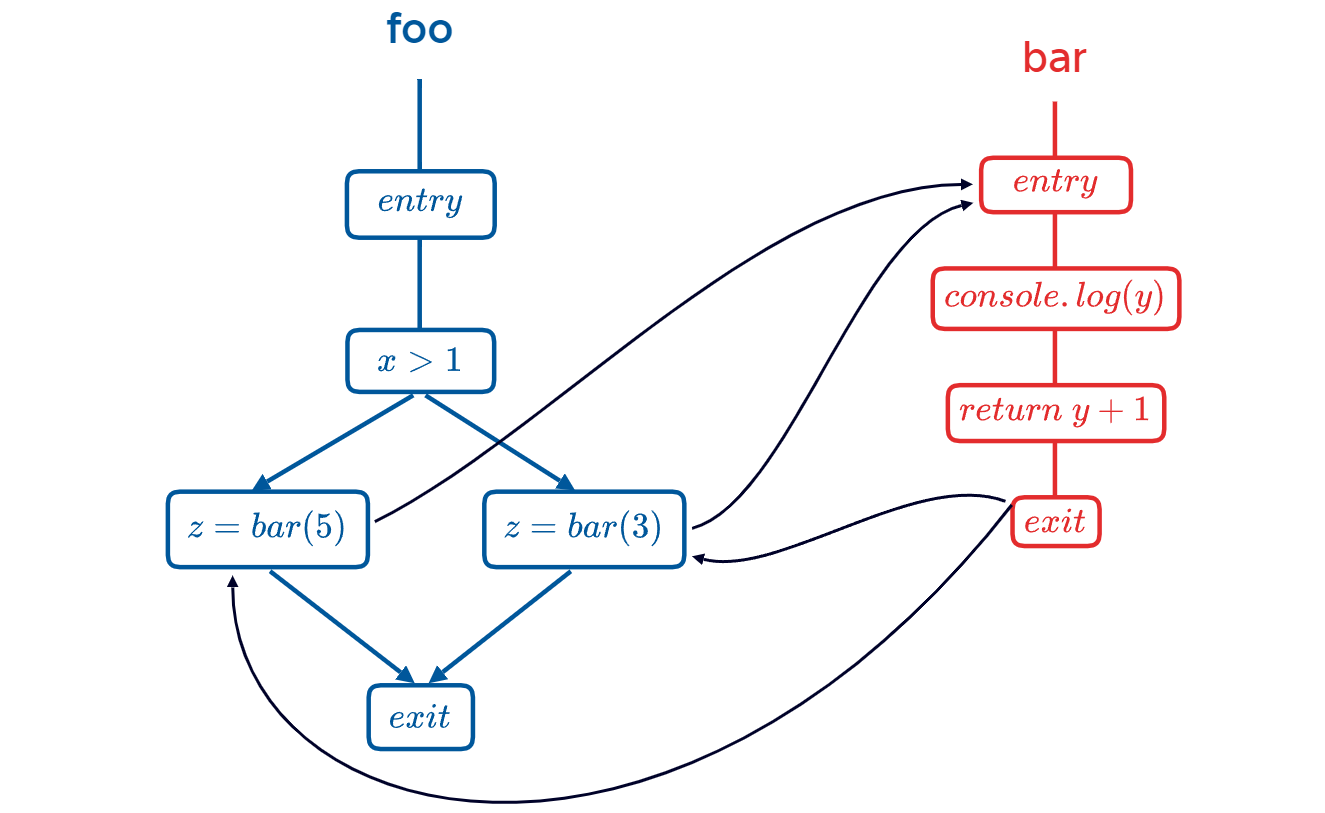
Example of inter-procedural control flow:

function foo(x) {
    if (x > 1) z = bar(5);
    else z = bar(3);
}
function bar(y) {
    console.log(y);
    return y + 1;
}

The control flow graph:

---

Information propagation in inter-procedural analysis:

• Arguments: propagate to formal parameters of callee
• Return value: propagate back to caller
• Local variable: do not propagate into callee, but when call returned, continue with the state just before the call

For inter-procedural backward analysis, everything mentioned above is in reverse.

3.6 Sensitivities

In static analysis, “sensitivity” is an important concept used to describe which kinds of information (e.g., order, paths, or contexts) an analysis distinguishes.

• Flow-sensitivity: takes into account the order of statements
• Path-sensitivity: takes into account the predicates at conditional branches
• Context-sensitivity (inter-procedural analysis only): takes into account the specific call site that leads into another function

---

Flow sensitivity - example:

if (...) {
    x = 3;
    x = 5;
}

In the context of flow-sensitive analysis, the value of x is designated as 5. Conversely, for flow-insensitive analysis, the value of x is 3 or 5, as the order of the statements is not largely considered.

---

Path sensitivity - example:

x = 0;
if (a > 0)
    x = 1;
else
    x = 2;
if (a > 0)
    x += 3;

Can x be 5? For path-sensitive analysis, the answer is no. But for path-insensitive analysis, the answer is yes, since it does not check whether the condition is satisfied.

---

Context sensitive - example:

n = 1;
function f(x) {
    if (x) {
        g(3);
    } else {
        n = 3;
        g(5);
    }
}
function g(y) {
    ...
}

Can n be equal to y? For context-sensitive analysis, the answer is no. But for context-insensitive analysis, the answer is yes.

---

Quiz: Consider an intra-procedural data flow analysis (specifically: live variables analysis). What sensitivities does it have?

sensitivity	answer
flow-sensitive	Yes (every data flow analysis)
path-sensitive	No (doesn’t track predicates)
context-sensitive	Irrelevant (it’s intra-procedural)

Footnotes

1. Non-trival properties are insidious, meaningful properties that describe significant program behaviors, such as “whether the program can terminate”, “whether the program always output 1”, while some properties like “whether the program contains 10 lines of code” is trivial for they are static properties, irrelevant to the runtime behaviors. ↩

2. A programming language is Turing complete such that it is capable of simulating any algorithm. Generally speaking, if a language can build branching, loops, recursion, and store and alter data, it is Turing-complete. ↩

3. This means that there does not exist a generalized algorithm that can determine non-trivial properties for all programs in a finite amount of time. ↩

4. Outgoing available expressions is the set of available expressions at a program point that are passed from that point. These expressions are available at that point and can be used by subsequent code (i.e., successor nodes to that point in the control flow graph). Incoming available expressions are the set of available expressions that are incoming from the preceding code (i.e., the predecessor node of that point in the control flow graph) at a program point. ↩

5. At first, I was actually confused about initial values. I thought that the information to start with the intermediate nodes ought to be $DF_{exit}(s_{i-1})$ but it is not. Nobody ever said that. Take available expressions analysis for example, it has $AE_{exit}(s)=(AE_{entry}(s)-kill(s))\cup gen(s)$, but $DF_{entry}(s)$ is not defined yet. ↩

6. Hoisting an expression: Pre-compute it, e.g., before entering a block, for later use. ↩