[SATV 0x08] Pointer Analysis

As a fundamental static analysis, pointer analysis computes which memory locations a pointer can refer to. For object-oriented programs (like Java), it mainly computes which objects a pointer (variables or fields) can refer to. Pointer analysis is often regarded as may-alias analysis, which is the focus of this lecture.

01 Alias Analysis

Alias analysis is the process of analyzing aliasing relationships between variables in a program, i.e., determining which variables may share the same memory address (or object). In a program, two or more variables are aliased if they point to the same memory address through mechanisms such as pointers, references, or arrays. The purpose of alias analysis is to understand the dependencies between variables, to avoid inconsistent accesses and modifications in the program, and to improve the readability and maintainability of the program.

There are two kinds of aliasing relationships—may-alias and must-alias. Let $a$ and $b$ be references to memory locations. At a program point $p$ :

$\mathrm{may-alias}(a,b)$ such that there exists at least one execution path to $p$ where $a$ and $b$ refer to the same memory location (or object).
$\mathrm{must-alias}(a,b)$ such that on all execution paths to $p$ , $a$ and $b$ refer to the same memory location (or object).

Example:

Circle x = new Circle();
Circle y = new Circle();
Circle t;
t = x;
x = y;
y = t;

This is a classic program for swapping two variables. In this program above, objects x and y are exchanged with each other. If it is analyzed using may-alias analysis, it can be obtained that there is a may-alias relationship between x and y, because in one of the program points x = y, x and y point to the same object; if it is analyzed using must-alias analysis, it can be obtained that there is no strict must-alias relationship between x and y because it does not exist on all execution paths.

It can be seen that may-alias analysis is just an approximation that provides a conservative analysis result, while must-alias analysis is more strict and precise.

May-alias analysis and must-alias analysis are duals of each other. But the technical machinery needed for must-alias analysis is far more advanced than that for may-alias analysis. Also, may-alias analysis is useful for many more practical data flow analysis problems than must-alias analysis. Therefore, in this lesson, we will focus on may-alias analysis, which is also called pointer analysis.

02 Pointer Analysis

The problem with pointer analysis is that it is undecidable. This means that we must sacrifice either soundness, completeness, or termination. We are going to compromise on completeness. In exchange for the possibility of false positives, we can design an alias-detection algorithm that terminates and never gives false negatives.

Let’s take a look at how a false positive manifests in this example. Suppose x MayAlias z returns Yes. Then, the most accurate information that our data-flow analysis can safely infer at this point is that x may or may not be equal to z. Conversely, if x MayAlias z returns No, then x and z cannot be aliases.

There are many sound approximate algorithms for pointer analysis with varying levels of precision. All these approximate algorithms generate false positives in certain circumstances, but they mainly differ in two key aspects:

How to abstract the heap (i.e. dynamically allocated data)
How to abstract control-flow

2.1 Abstractions

Let’s dive deeper into data and control-flow abstractions for pointer analysis using an example program.

void doit(int M, int N) {
    Elevator v = new Elevator();
    
    v.floors = new Object[M];
    v.events = new Object[N];
    
    for (int i = 0; i < M; i++) {
        Floor f = new Floor();
        v.floors[i] = f;
    }
    
    for (int i = 0; i < N; i++) {
        Event e = new Event();
        v.events[i] = e;
    }
}

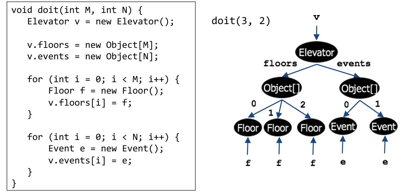
Throughout this lesson, we will use this Java program to illustrate the key concepts of pointer analysis. This program constructs a representation of an elevator.

An Elevator object has two fields.

One field is an array of Floor objects (points to the floors field) representing different floors in a building, such as the basement, 1st floor, 2nd floor, and so on.

The other field is an array of Event objects (points to the events field). An example event is a person pushing a button for the 2nd floor in an elevator currently on the 5th floor.

The doit function takes as input the number of floors M and the number of events N. It starts out by creating an object of class Elevator. It then initializes the floors and events fields of the created Elevator object.

Let’s assume that the doit function is called with M=3 and N=2. The graph below represents the points-to relationships in this concrete run of the program.

2.1.1 Abstracting the Heap

This run for the elevator program created only three floors and two events, but a pointer analysis must be able to reason about each run with M floors and N events for any value of M and N.

Pointer analysis achieves this by abstracting the heap. There are many possible schemes to abstract the heap, each of which strikes a different tradeoff between precision and efficiency. One of these schemes abstracts objects based on the site at which they are allocated in the program.

The elevator program has five allocation sites. Therefore, pointer analysis operates on the following graph, which conflates all objects allocated at the same site into a single node of the graph.

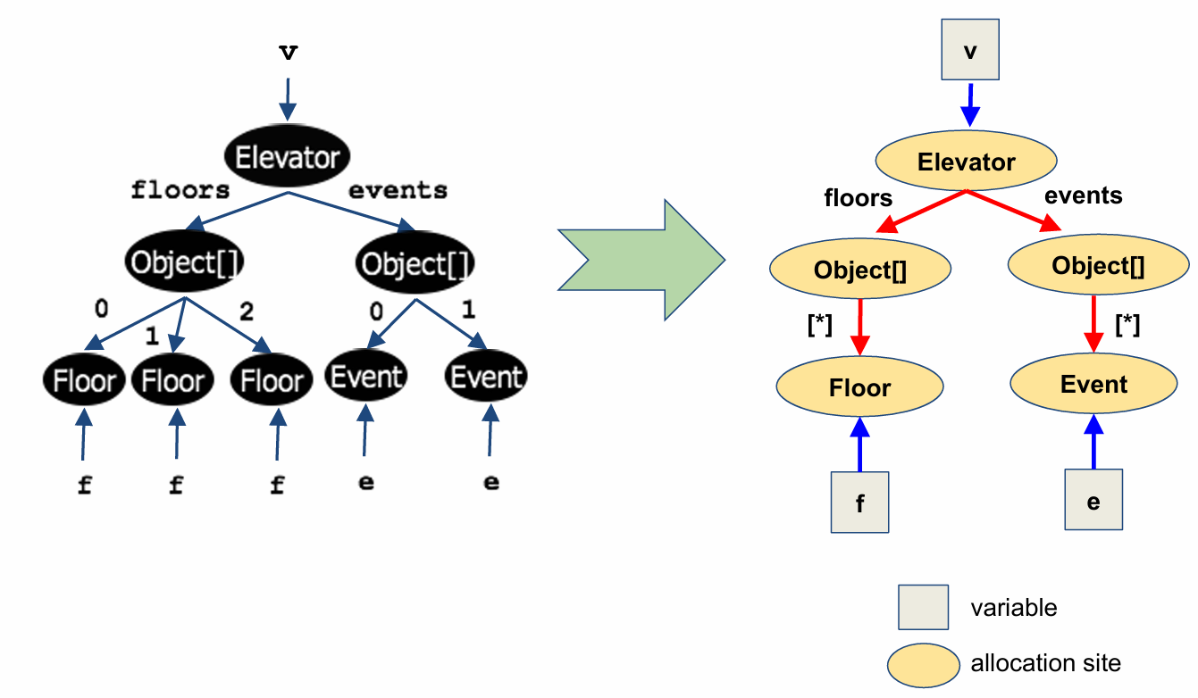
In particular, it collapses all the Floor nodes into a single Floor node, and all the Event nodes into a single Event node. Instead of labeling the pointers from the Object array nodes to these individual objects by array indices, we use the nondeterministic-choice symbol asterisk and also observe that the variables f and e now point to a single node each instead of multiple nodes.

The type of graph that this heap abstraction produces is called a “points-to” graph. In a general points-to graph, there are two kinds of nodes: variables and allocation sites. Variables will be denoted by boxes, and allocation sites will be represented by ovals. A core task of pointer analysis is to construct such a points-to graph.

Since the points-to graph relation is an asymmetric relationship (that is, pointers between data need not go both ways), this is a directed graph. So we will represent edges with arrows. There are two types of edges in this graph. Arrows from a variable node to an allocation site node will be colored blue, and arrows from one allocation site node to another allocation site node will be colored red and labeled by a field name.

2.1.2 Abstracting Control-Flow (Flow Insensitivity)

Although points-to graphs are finite, it is too expensive in practice to track a separate such graph at each program point. Most pointer analyses only track a single, global points-to graph for the entire program. They achieve this by abstracting control-flow.

The particular control-flow abstraction that is commonly used by pointer analyses is called flow insensitivity. Applying this abstraction to our example elevator program produces the following abstract program.

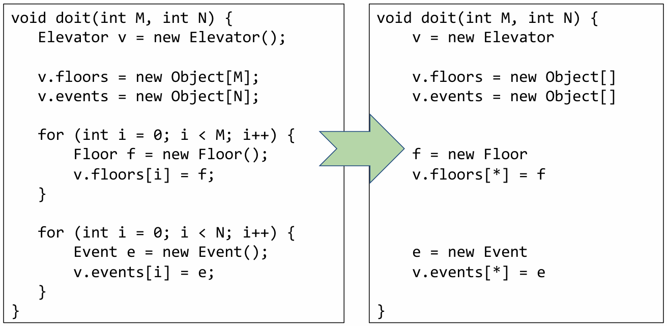
There are three major differences I’d like to highlight here:

Notice that all control-flow features have been removed, including constructs like for-loops and also semicolons indicating sequentially ordered statements.
All statements that do not affect pointers have also been removed. For example, the approximated code no longer has statements setting the integer i equal to 0 and incrementing i.
Finally, array indices are replaced by nondeterministic choice, denoted by the asterisk symbol.

This abstraction can be thought of as turning the program into an unordered set of statements. Even though we’ve written the statements in the rough order they appear in the original program, it is better to think about the statements as having no precedence over each other.

Even though this abstraction appears to lose a lot of information, we will see later in this lesson that it is still able to prove interesting properties, such as the property that variables e and f do not alias.

Next, let’s see how a pointer analysis algorithm builds a points-to graph for an arbitrary program.

2.2 A Simple Language

For pointer analysis, it suffices to consider the following kinds of statements:

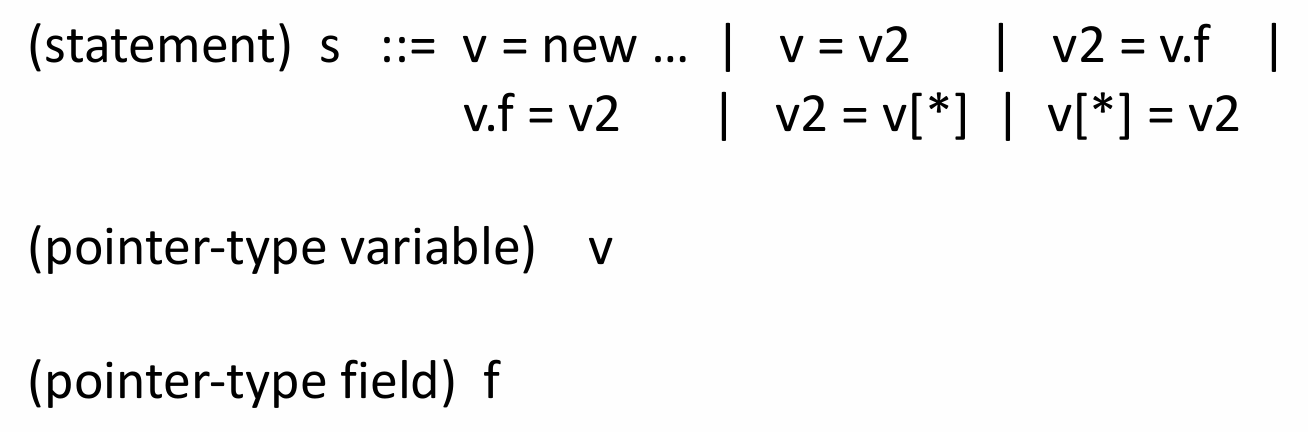
First, we must consider object allocation statements that create pointers using the new keyword. This is exemplified in the above figure by v=new ....

In addition to pointer creation, we also must consider when a variable aliases that pointer. This situation is shown by the assignment v=v2. We call this an “object-copy” statement because the memory address referring to an object is copied from v2 to v.

Next, we must consider field-reads and field-writes. These statements use the dot operator to access fields on an object. This is exemplified in the above figure by v2=v.f.

Lastly, we must consider the case in which array members alias pointers. In other words, when an array holds pointers to an object. We consider both cases in which we read and write to these members. These are exemplified in the above figure by v2=v[*] and v[*]=v2.

At this point, you might be wondering whether the grammar we just presented is sufficient to represent all the operations that we might need to reason about in order to determine whether two pointers may alias. The answer is yes.

We will not give a formal proof of this fact in this lecture. However, you can convince yourself this is sufficient by the intuition that all of the ways in which aliasing can occur are covered by this grammar.

We will now go through some examples of how to break down more complicated statements into compositions of these six simpler types of statements.

First, let’s consider the statement v.events = new Object[] from our elevator program. This statement starts with an allocation of the Object array, and then it assigns the address of the new allocation to the field events of the Elevator object. We can break this statement down into a field write and an object allocation, which are:

tmp = new Object[]
v.events = tmp

Now, let’s consider our second example, v.events[*] = e. It performs a read of the events field of the Elevator object, and then it assigns the content of e to some cell in the Object array that v.events points to. We can again break this statement up into two separate statements of the forms above, which are:

tmp = v.events
tmp[*] = e

It is now clear that complex statements involving pointer aliasing can be broken into two simple statements of the form specified in our grammar.

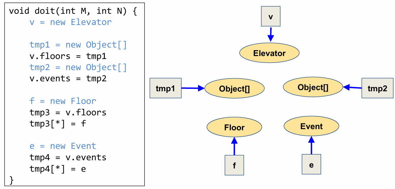
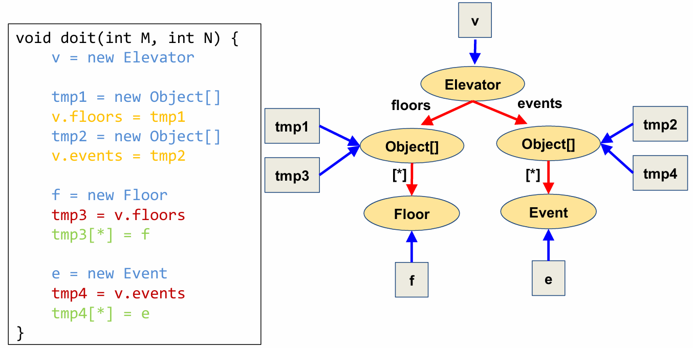
Finally, let’s decompose the statements in our Elevator program and we obtain:

void doit(int M, int N) {
	v = new Elevator

	tmp1 = new Object[]
	v.floors = tmp1
	tmp2 = new Object[]
	v.events = tmp2

	f = new Floor
	tmp3 = v.floors
	tmp3[*] = f

	e = new Event
	tmp4 = v.events
	tmp4[*] = e
}

Quiz: Convert each of these two expressions to normal form:

// Q1
v1.f = v2.f
// Q2
v1.f.g = v2.h

Answer:

// A1
tmp = v2.f
v1.f = tmp
// A2
tmp1 = v1.f
tmp2 = v2.h
tmp1.g = tmp2

2.3 Andersen’s Algorithm

One of the most well-known pointer analysis algorithms is Andersen’s algorithm. The algorithm, that builds the points-to graph for a given program, was published in 1994. Note that the structure of the algorithm is similar to the Worklist algorithms that we presented in the dataflow analysis module.

graph = empty
repeat:
	for (each statement s in program)
		apply rule corresponding to s on graph
until graph stops changing

Starting with an empty graph, we examine statements that create pointers and update the graph based on points-to-relationships. The algorithm terminates when the graph stops changing.

The set of statements that we iterate over is obtained using the flow-insensitive abstraction we just presented. In addition to removing control flow, we also removed any statements that did not “affect pointers.” Let’s dive into the details of which statements are included.

2.3.1 Rule for Object Allocation

By now, you should be convinced that we can take a program written in our simplified Java-like language and express its pointer operations using the six simple statements we introduced earlier.

In order to perform Andersen’s algorithm, we need to understand how each type of statement affects the points-to-graph. The graph is updated depending on the type of statement currently being analyzed.

To make things more concrete, let’s see how an object allocation statement affects points to relations.

For a statement v=new B, we create a new allocation site node called B, we create a variable node for v (if it doesn’t already exist), and then add a blue arrow from the variable node to the allocation site node.

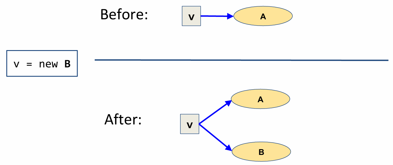
Note that if there is already an arrow from v to another allocation site node (say A), we just need to add a new arrow from v to B. This rule, as well as all the remaining rules we’ll discuss, is a “weak update,” in which we accumulate instead of replace the points-to information (which would be a “strong update”). This type of update rule is a hallmark of flow-insensitivity.

Looking at our example Elevator program, let’s use the object allocation sites rule to create a partial points-to-graph.

2.3.2 Rule for Object Copy

Now, let’s expand our points-to-graph to include a few more relationships.

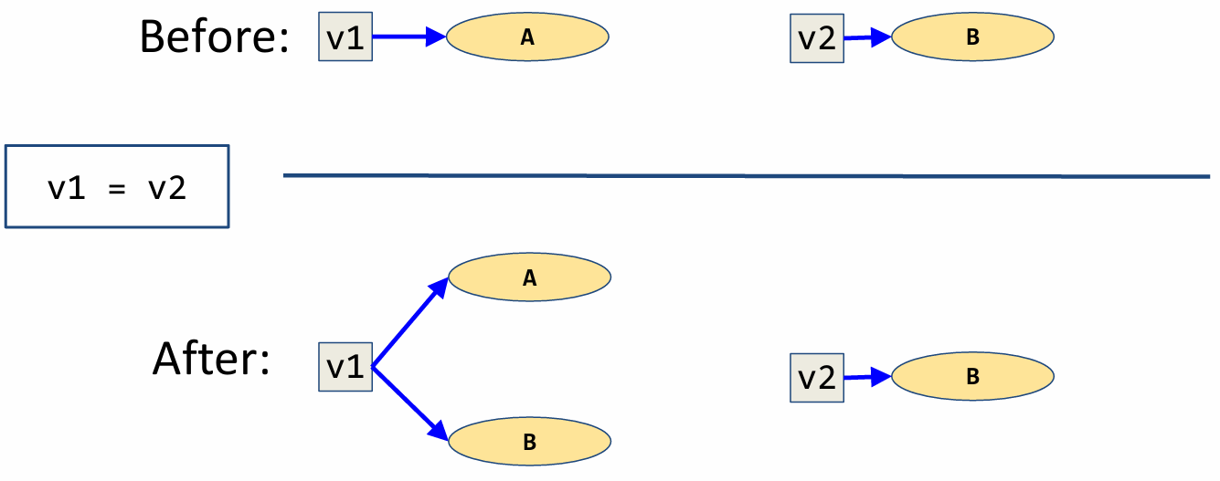
First, let’s add alias relationships created through “object copy.”

For the statement v1 = v2, we create a variable node for v1 (if it doesn’t already exist), and then add a blue arrow from the variable node for v1 to all nodes pointed to by the variable node for v2.

Again note that we do not remove or replace any existing arrows from v1. v1 merely accumulates another arrow to B.

In words, v1 now additionally points to what v2 points to.

2.3.3 Rule for Field Writes

Now, let’s see how field writes affect relationship in a points-to-graph. Field-write statements can be one of the following forms.

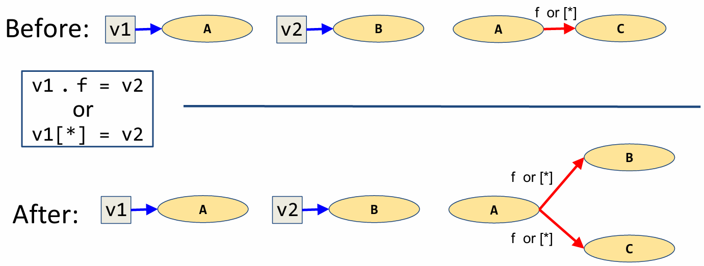
Although the two statements shown here are syntactically different, they will have the same affect on a points-to graph.

Prior to the field write statement, suppose v1 points to A and v2 points to B. Additionally, A has a link between its allocation site and the allocation site for the field f, or equivalently, the array member denoted by [*]. This represents the portion of memory specifically reserved for the field or array member.

The field write statement modifies the points-to-graph by adding a field relationship, denoted by a red arrow, from A to the value stored in v2. That is, we add a red arrow from A to B. Again, we perform a “weak update” and do not remove the field relationship between A and C.

Now, there are some edge cases we must consider. For instance, what should we do if v1 and v2 point to the same node? This would be equivalent to the statement v1.f=v1. As you might have guessed, we will add a red arrow from A to itself.

As another edge case, what should we do if there isn’t already a node for v1 or v2? In this case, we should skip this statement temporarily and handle it in the next iteration.

Now let’s update our points-to-graph for the elevator program by applying the field-write update rule.

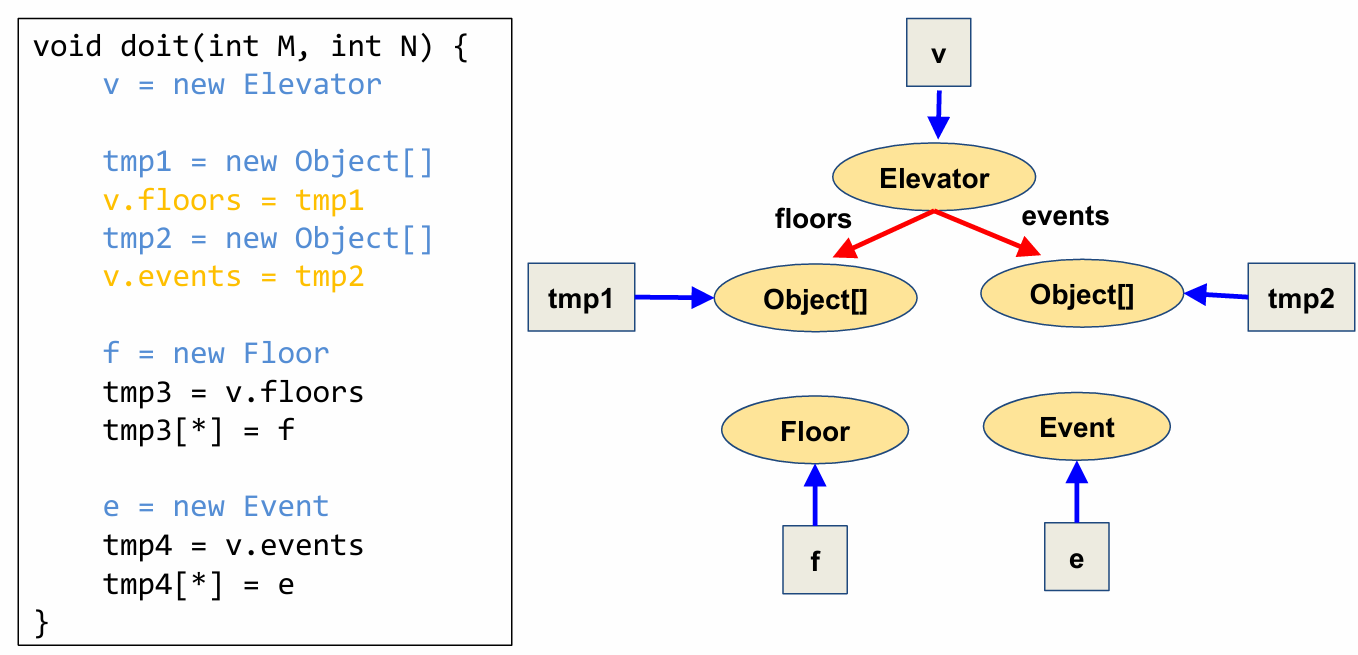
The latter two field-writes (tmp3[*]=f and tmp4[*]=e) in this program are through arrays. However, since the variables nodes for tmp3 and tmp4 haven’t been created yet, we skip these field-write operations and will come back to them in a later iteration.

2.3.4 Rule of Field Reads

Now, let’s see how field-read relationships update a points-to-graph. As in field-writes, field-reads also have an equivalent rule update for reads from array members.

Suppose we have the setup shown here prior to the field-read statement. That is, v1 points to the allocation site A, V2 points to the allocation site B, and B has a link to C denoting field f, or, equivalently, array access [*].

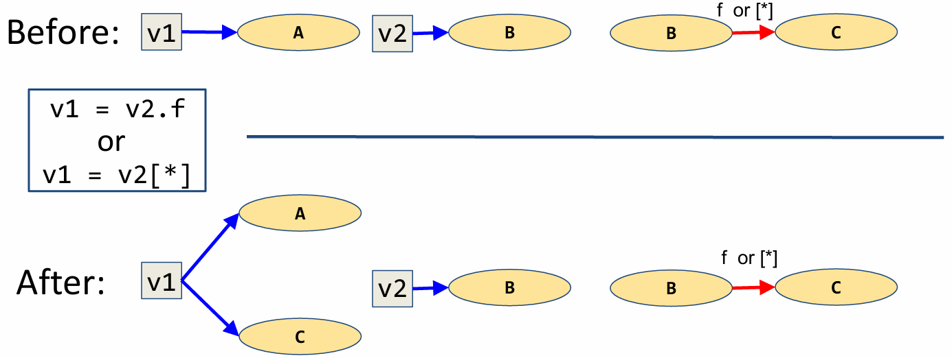
Field-reads, in themselves, do not modify any points-to relationships. However, an assignment to a field read, can indeed modify relationships and thus will have an affect on our points-to-graph.

Following the shown field-read assignment, the variable v1 now points to the allocation site for field f (or array member [*]) of the object pointed to by v2. So, we add a arrow from v1 to C by following the arrows representing field relationships.

As in all update rules, we perform a “weak update” and keep the points to relationship between v1 and A. Note that object B may in fact be pointing to many other objects via arrows labeled by the field in question. In this case we would need to add an arrow from v1 to each of these nodes in order to reflect the fact that the field f, and therefore v1, may point to any one of these objects.

Lastly, we must consider the case in which the variable nodes for v1 or v2 do not exist. As you might guess, we skip the statement temporarily and try to handle it in the next iteration. Likewise, if there is no field relationship from B via f or [*], we skip the statement for this iteration.

Now let’s extend our points-to-graph for the elevator program by applying the field-read update rule.

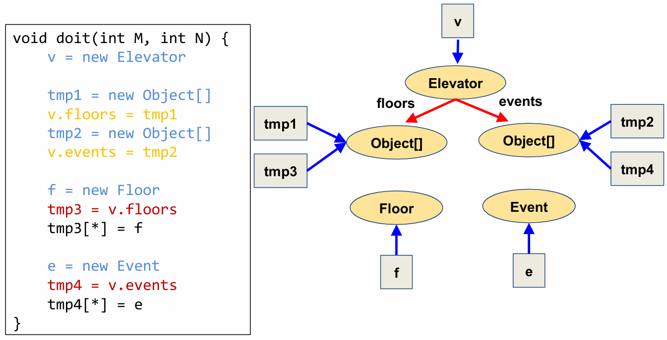
Now that we’ve created nodes for tmp3 and tmp4, we can apply the field-write rules to the statements we skipped previously.

03 Dimensions of Pointer Analysis

Andersen’s algorithm is one example of a pointer analysis. As with other analyses, points-to analysis has many different “knobs” that we can tune for increasing precision or efficiency. However, an increase in precision usually comes at a cost in efficiency.

We can classify a points-to analysis algorithm across many different dimensions. Each dimension allows the reader to understand, at a high level, how the algorithm balances precision and efficiency.

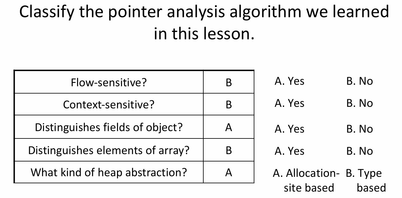
In order to classify a given analysis across four dimensions, we can ask the following questions:

Does the analysis consider control flow (or is it flow-sensitive)?
Does the analysis analyze a single function or an entire program at once (or is it context-sensitive)?
How does the analysis abstract the heap (or what heap abstraction scheme is used)?
How are aggregate data types such as records or classes modeled (or how are aggregate data types modeled)?

Let’s discuss each of these four dimensions more deeply.

3.1 Flow Sensitivity

Flow-sensitivity concerns how a pointer analysis algorithm models control-flow within a procedure or function. As we are only concerned with control flow within each function, we call this intra-procedural control flow. We can classify an analysis based on how it models control flow within a function as flow-insensitive or flow-sensitive.

Flow-insensitive pointer analysis algorithms, like the one we just discussed, ignore control-flow entirely, viewing the program as an unordered set of statements. A hallmark of flow-insensitive analyses is that these analyses only generate new facts as they progress; they never kill any previously generated facts. We observed this in the case of the pointer analysis algorithm we just saw, wherein the points-to graph only grew in size as each statement of the program was considered. We say that such algorithms perform weak updates. Such algorithms typically suffice for may-alias analysis, that is, it is practical for a may-alias analysis to have a low false positive rate despite being flow-insensitive.

Flow-sensitive pointer analysis algorithms, on the other hand, are capable of killing facts in addition to generating facts. We say that such algorithms perform strong updates. This is possible as we have a distinct program order in which facts that come later take precedence over facts generated earlier in the program order. Such algorithms are typically required for must-alias analysis, that is, it is impractical for a must-alias analysis to have a low false positive rate by being flow-insensitive.

3.2 Context Sensitivity

Another common dimension for classifying pointer analysis algorithms is context sensitivity, which concerns how to handle control-flow across procedures. This property is called inter-procedural control-flow. We can classify pointer analysis algorithms as context-insensitive or context-sensitive, based on how they handle inter-procedural control-flow.

Context-insensitive pointer analysis algorithms analyze each procedure once, regardless of how many different parts of the program call that procedure. These algorithms are relatively imprecise, as they conflate together aliasing facts that arise from different calling contexts. But they are very efficient, since they analyze each procedure only once.

Context-sensitive pointer analysis algorithms, on the other hand, potentially analyze each procedure multiple times, once per abstract calling context. These algorithms are relatively precise but expensive. They differ primarily in the manner in which they abstract the calling context. Like many choices in analysis, the choice of the scheme is dictated by the desired tradeoff between precision and efficiency.

3.3 Heap Abstraction

In addition to abstractions in control flow, pointer analyses may also have various levels of abstraction for dynamic memory. A heap abstraction concerns abstracting program data, in particular, dynamically allocated objects on the heap.

As we saw earlier in the lesson, keeping track of aliasing without abstractions can be expensive or even infeasible. In order to lessen this burden, analyses often create an abstraction of the dynamic allocation sites. A heap abstraction scheme specifies how to map a potentially infinite number of concrete dynamically allocated objects to a finite number of abstract objects. Each abstract object corresponds to an oval node in the points-to graph. This partitioning is at the heart of ensuring that pointer analysis terminates.

Much like any of the abstractions we have seen in this course, designing a suitable heap abstraction is an art. Many sound heap abstraction schemes exist with varying precision and efficiency. As a rule of thumb, a scheme that produces too few abstract objects in the points-to graph will result in an efficient but imprecise pointer analysis - imprecise because it conflates more concrete objects into each of the few abstract objects. On the other hand, a scheme that produces too many abstract objects in the points-to graph will result in an expensive but precise pointer analysis.

Let’s take a look at three heap abstraction schemes that are commonly used from most precise to least precise.

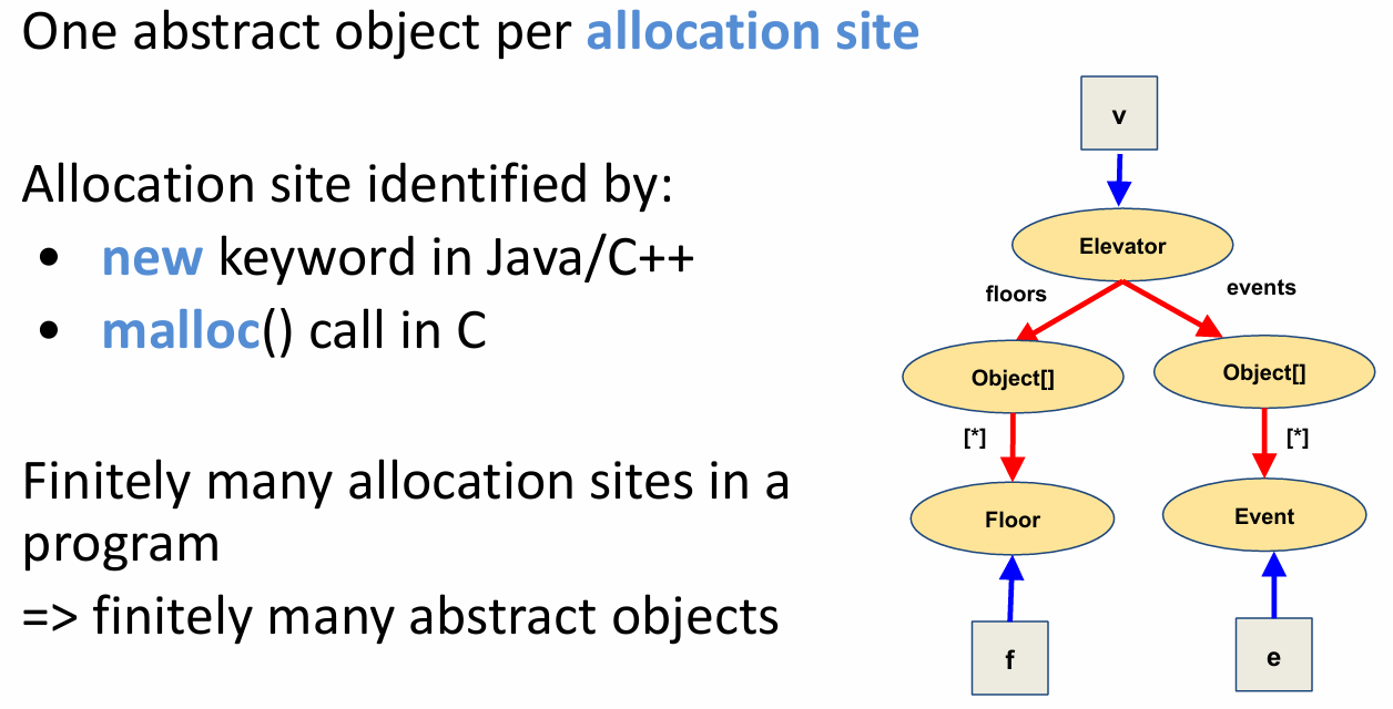
3.3.1 Allocation-Site Based

The heap abstraction scheme used by Andersen’s algorithm that we illustrated in this lesson is called the allocation-site based scheme. This scheme abstracts concrete objects based on the site in the program where they are created, called the allocation site. In other words, each abstract object under this scheme corresponds to a separate allocation site.

Allocation sites are identified by the new keyword in Java and C++, and by the malloc function call in C. Since there are finitely many allocation sites in a program, a pointer analysis using this scheme is guaranteed to result in a finite number of abstract objects in the constructed points-to graph.

Here is the points-to graph that was constructed using the allocation-site based scheme for our example elevator program. Each of the five ovals correspond to a separate allocation site in the program.

3.3.2 Type Based

Now let’s consider a slightly less precise scheme based on types. Although the number of allocation sites in any program is finite, tracking a separate abstract object per allocation site can be prohibitively expensive for large programs, which can contain too many allocation sites.

This scheme partitions concrete objects based on their type instead of based on the site where they are created. In other words, each abstract object under this scheme corresponds to a separate type. Since there are finitely many types in a program, a pointer analysis using this scheme is guaranteed to result in a finite number of abstract objects in the constructed points-to graph.

Here is the points-to graph that would be computed for our example elevator program by a pointer analysis using the type-based scheme. Notice that each of the four ovals corresponds to a separate type in the program. In particular, notice that the two separate ovals that were created for the arrays of floors and events are now conflated into one, as both have the same type: an array of objects.

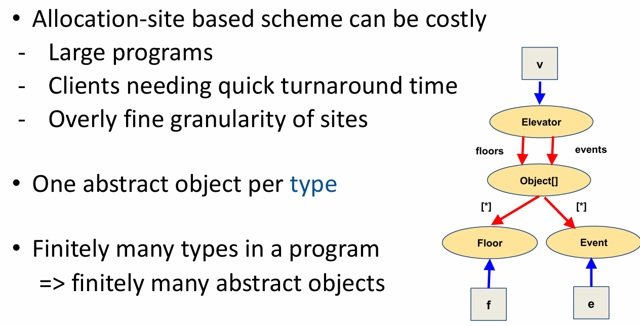
This scheme may be appealing to clients of pointer analysis that need a quick turnaround time to aliasing queries, such as an integrated development environment.

3.3.3 Heap-Insensitive

Now let’s consider an even more imprecise abstraction scheme.

In this scheme, we do not make any distinctions between dynamically allocated objects. We call this “heap-insensitive”. This scheme uses a single abstract object to model the entire heap.

The points-to graph for our example elevator program is shown here. It contains a single abstract node for the entire heap. Looking at this points-to graph, it should be easy to see that this scheme is highly imprecise for reasoning about the heap, but it is sound nevertheless.

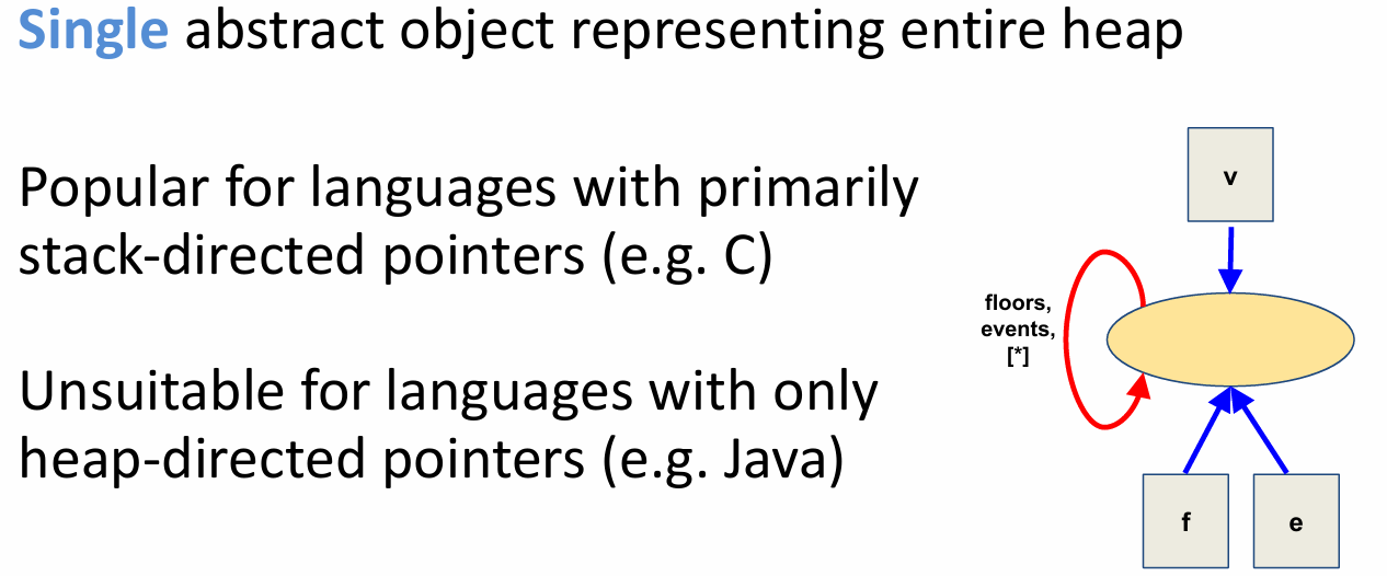
So you might wonder: are there scenarios in which this scheme is useful? The answer is yes, for languages with primarily stack-directed pointers like C, where malloc calls are sparse. Pointer analyses for such languages derive most of their precision by reasoning about stack-directed pointers, and completely ignoring heap-directed pointers.

Of course, this scheme is unsuitable for languages with only heap-directed pointers like Java.

We will look at pointer analyses for programs with stack-directed pointers later in this module.

3.3.4 Summary

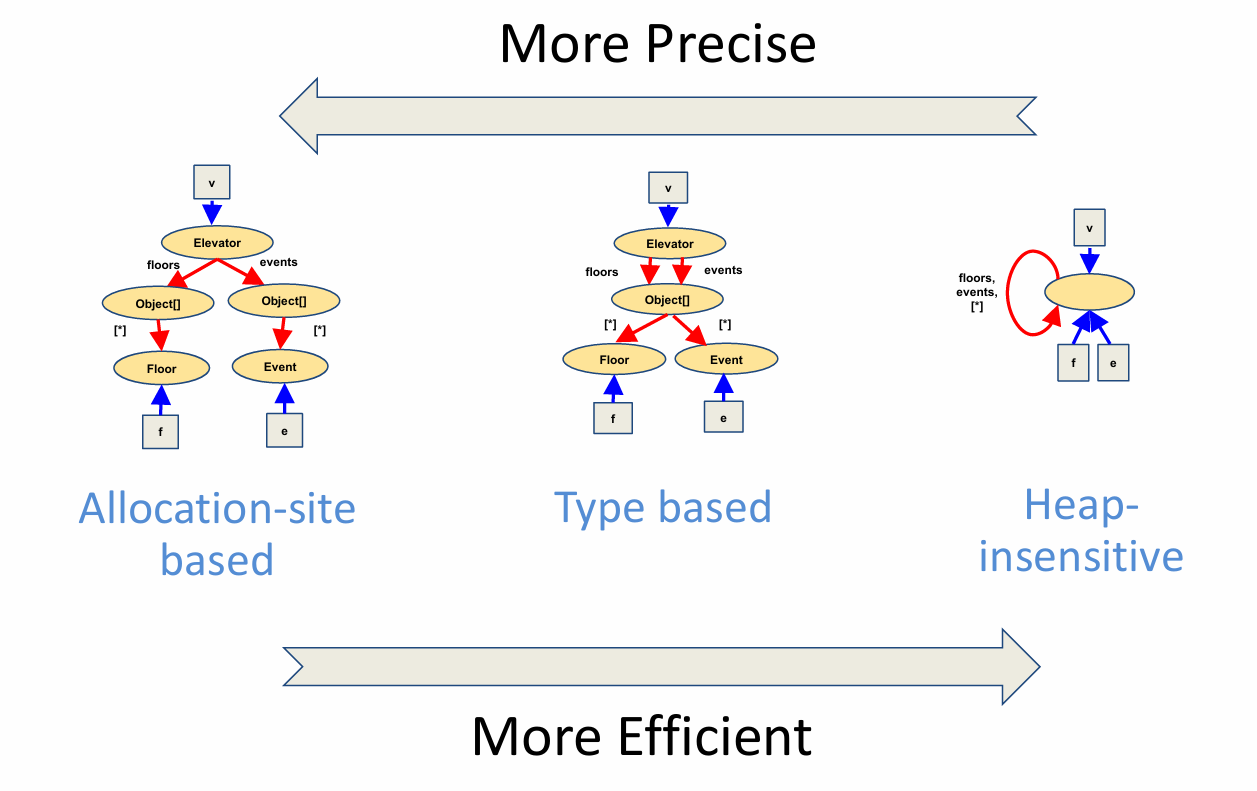
To recap, the three different heap abstraction schemes that we just saw strike a different tradeoff between precision and efficiency. As we go from the allocation-site based scheme to the type-based scheme to the heap-insensitive scheme, the pointer analysis gets more efficient, but also less precise.

It is important to remember that these are not the only three schemes: there are many other schemes in the literature, and you can even design your own depending on your analysis needs. For instance, there are many schemes that are more expensive and precise than the allocation-site based scheme; these schemes can even make distinctions between objects created at the same allocation site. At the same time, remember that we can never have a scheme that will allow pointer analysis to make distinctions between all concrete objects and terminate in finite time.

3.4 Modeling Aggregate Data Types

Another dimension for abstracting program data in a pointer analysis concerns how to model aggregate data types. These include arrays and records. Let’s look at arrays first.

3.4.1 Arrays

A common choice in pointer analyses is to use a single field, denoted by asterisk, to represent all elements of an array. Such analyses therefore cannot distinguish between different elements of an array. The pointer analysis algorithm we saw earlier in this lesson uses this representation.

More sophisticated representations make distinctions between different elements of an array. Such representations are employed in so-called array dependence analyses whose primary goal is to determine whether two integer expressions refer to the same element of an array, much like the primary goal of pointer analysis is to determine whether two pointer expressions alias.

Array dependence analysis is used in parallelizing compilers to parallelize sequential loops.

3.4.2 Records

Now let’s look at another common kind of aggregate data type: records.

Records are also known as structs in C or classes in object-oriented languages like C++ and Java.

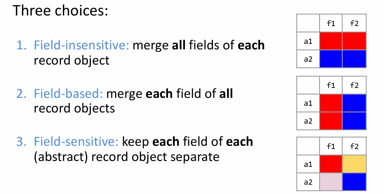
There are three common choices that pointer analyses use to model records.

We will illustrate these three choices using a record type with two fields f1 and f2. Suppose there are two objects a1 and a2 of this record type.

The first option shown here is a field-insensitive representation. The abstract state merges all fields of each record object. In other words, this representation prevents the analysis from distinguishing between different fields, such as f1 and f2, of the same record object, such as a1 or a2.

Another choice is to use a so-called field-based representation, which merges each field across all record objects. In other words, this representation prevents the analysis from distinguishing between the same field, such as f1 or f2, of different objects, such as a1 and a2.

The third choice is to use a field-sensitive representation, which keeps each field of each abstract record object separate. Assuming that a1 and a2 denote distinct abstract objects, this representation allows the analysis to distinguish all four memory locations denoted by this table: field f1 of a1, field f2 of a1, field f1 of a2, and field f2 of a2. It is easy to see that this is the most precise of the three representations. The pointer analysis algorithm we studied earlier in this module used this representation.

Let’s reflect on the pointer analysis we looked at. Classify it according to the dimensions we just discussed.