[SATV 0x09] Taint Analysis

01 Information Flow Analysis

Taint Analysis is an application of Information Flow Analysis. Therefore, we will first give a introduction of information flow analysis before returning to the topic of taint analysis.

1.1 Introduction

Information flow analysis is a kind of analysis that is typically used in the context of security, where the overall goal is to secure the computing system. Specifically, the goal of information flow analysis is to do this by securing the data manipulated by a computing system and by enforcing a particular security policy:

• Confidentiality: Secret data does not leak to non-secret places
• Integrity: High-integrity data is not influenced by low-integrity data¹

Confidentiality and integrity are dual problems for information flow analysis.

The way an information flow analysis checks whether there could be a violation of a confidentiality or an integrity policy is by checking whether information may propagate from one “place” (e.g. a code location or variable) in the program propagates to another “place” in the program.

Information for analysis is only about how data and information propagate within a program. Thus it often complements techniques that impose limits on releasing information, such as access control lists and cryptography. These security mechanisms check other kinds of properties in particular that are responsible for making sure that information is only released in a controlled way. This, however, is not what information flow analysis is really about.

Let me give a simple example of confidentiality and integrity.

Imagine that there is a place in the program that holds some secret information, such as a password or a credit card number, which you know it is not supposed to reach other places that are untrusted or unsafe. Now, one thing that information flow analysis is going to do is to check whether it’s possible that the secret information may flow to other places that you know to be untrusted. And if it really does, it is checking a confidentiality policy.

The inverse to confidentiality policies are integrity policies where we also have some untrusted places and in addition we have some places in which we’re going to store trusted information. So, another thing that information flow analysis is going to do is to check whether it’s possible that there is a flow of information from the untrusted places to the places that store trusted information. If it really does that, it is checking a integrity policy.

---

Here are two more concrete examples for confidentiality and integrity, respectively.

Example 1: Confidentiality

var creditCardNb = 1234;
var x = creditCardNb;
var visible = false;
if (x > 1000) {
	visible = true;
}

In this program, the credit card number (stored in creditCardNb) is secret information that should not leak to non-secret places. However, it propagates to x in line 3 and partly propagates to visible in line 5, compromising the policy of confidentiality.

Example 2: Integrity

var designatedPresident = "Michael";
var x = userInput();
var designatedPresident = x;

userInput should not influence who becomes the president, at least not before being certified. However, it is passed to designatedPresident, which is apparently a high-integrity variable, thereby breaking the policy of integrity.

1.2 Tracking Security Labels

Now we know what information flow analysis is going to do, so the next question is how to analyze the flow of information through a program. The key idea is tracking the so-called security labels.

Security labels are some meta information assigned to each value, which tracks the secrecy of the value. And whenever some program operation happens, or whenever we are computing a new value from some old values, then we are propagating the meta information so that in the end we know for every value in the program what level of secrecy this value has.

---

Example: Tracking Security Labels

var creditCardNb = 1234;	// secret
var x = creditCardNb;
var visible = false;
if (x > 1000) {
	visible = true;
}

As we have discussed before, creditCardNb carries secret information and is therefore assigned some meta information indicating that this value is secret. In line 2, the value of creditCardNb propagates to x through the execution of the program, and so does its meta information. In line 4, it has a condition x>1000. Although this statement does not propagate secret information to other variables entirely, it partially leaks information to visible, which makes it possible for attackers to determine whether the value of x is greater than 1000 based on the value of visible.

1.3 Non-Interference

Instead of defining what the analysis is supposed to do by talking about the propagation of individual pieces of data from one place in the program to another, we can also try to formulate this as a property of the entire program, and this is what this notion of Non-Interference that I’m talking about is doing.

Essentially, what non-interference means is that “Confidential data does not interfere with public data.” Specifically, it means that:

• Variation of confidential input does not cause a variation of public output
• Attacker cannot observe any difference between two executions that differ only in their confidential input

1.4 Lattice of Security Labels

So far in the previous examples, we have basically two levels of secrecy - one was public and the other was private. Of course we can generalize this idea to more levels of secrecy and this is what we are going to do next.

1.4.1 Example

In this part, we will look at a lattice composed of a set of security labels, which are combined in a way that they form a so-called universally bounded lattice. It’s a way to define different levels of security and define what happens if information that have different levels of security are combined with each other so that you know what level of security you’ll get in the combined value.

Let’s start by showing a few examples of these lattices before we define formally our lattice.

In the previous examples, we have only two security classes called high and low. However, if you have different levels of people who may have different kinds of information and you want different security levels to represent that hierarchy, then two classes may not be enough.

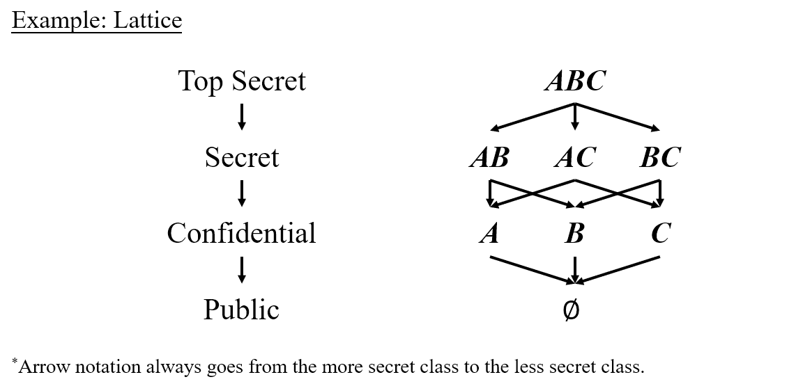
One way to do so is to basically define multiple such security classes where one is always more secret than the other one. So let’s say we have four security classes this time, among which top secret is the most secret, followed successively by secret, confidential and public. We use arrow notation to connect these different classes and the arrows always go from the more secret class to the less secret class.

Maybe this stacked set of security labels is still not enough because sometimes we want to express that we need different kinds of permissions in order to see a piece of information, and different people or different parts of a program may have different subsets of these permissions. Sounds complicated right? We can do this by the so-called subset letters. We define three different kinds of permissions $A$, $B$, $C$, which, if you have all of them, grant you top access to information of all security levels. Maybe some parts of the program only have some subset of this larger set, for example $AB$, $BC$, $AC$, which are at a lower level than $ABC$ because you are allowed to see less information. Of course you may just have one of them which gives you a even lower level. Considering that $A$ is the subset of both $AB$ and $AC$, we will connect them simultaneously, and so are $B$ and $C$. However, this isn’t the end. At the bottom of this hierarchy, we have $\emptyset$, which gives you no permission to see anything.

The following figure shows the example we have just depicted.

1.4.2 Universally Bounded Lattice

The lattice we have just exemplified is called a Universally Bounded Lattice. Now, we are going to formally define it.

$$\text{Universally Bounded Lattice: }Tuple(s,\rightarrow,\bot,\top,\oplus,\otimes)$$

The above formulation gives the formal definition of a universally bounded lattice. Such a universally bounded lattice is a tuple that consists of six parts:

• $s$: a set of security classes
• $\rightarrow$: a partial order between these classes
• $\bot$: the lower bound
• $\top$: the upper bound
• $\oplus$: the least upper bound operator - takes the union of sets, e.g., $A\oplus BC=ABC$
• $\otimes$: the greatest lower bound operator - takes the intersection of sets, e.g., $A\otimes AB=A$

Let’s use this definition to define the example we’ve just introduced:

• $s$: $\{ABC,AB,BC,AC,A,B,C,\emptyset\}$
• $\rightarrow$: $\{ABC\rightarrow AB,ABC\rightarrow AC,ABC\rightarrow BC,AB\rightarrow A,AB\rightarrow B,BC\rightarrow B,BC\rightarrow C,AC\rightarrow A,AC\rightarrow C,A\rightarrow\emptyset,B\rightarrow\emptyset,C\rightarrow\emptyset\}$
• $\bot$: $\{\emptyset\}$
• $\top$: $\{ABC\}$
• $\oplus$: $s\oplus s\rightarrow s$
• $\otimes$: $s\otimes s\rightarrow s$

02 Taint Analysis

Now that we have established a basic grasp on information flow analysis, we can proceed to taint analysis.

The goal of taint analysis is to analyze the propagation of tainted data to ensure data integrity and confidentiality. Its theoretical foundations are as follows:

• The lattice model: $(SC,\preceq)$² where $SC=\{Tainted,Untainted\}$
• If information is propagated from a variable of type Tainted to a variable of type Untainted, then the data of type Untainted needs to be changed to type Tainted.
• If a variable of type Tainted is passed to an important data area or an information leakage point, it means that the information flow policy has been violated.

2.1 The Heartbleed Vulnerability

We will begin with a famous bug, known as the heartbleed vulnerability, in OpenSSL to examplify the application of taint analysis in practice.

OpenSSL is an encryption-related library that is widely used to protect communications over the Internet, including connections to websites and email servers. If a system is using a vulnerable version of OpenSSL, the heartbleed vulnerability can be used to leak information about that system. This could contain highly sensitive information such as private keys and usernames/passwords stored in memory.

The heartbleed vulnerability implements a typical buffer overflow vulnerability using OpenSSL’s Heartbeat protocol (note that Heartbeat is the name of the exploited protocol, while Heartbleed is the name of the vulnerability). The Heartbeat protocol allows a device to check whether a connection to a Secure Sockets Layer (SSL) enabled server is still alive by sending a heartbeat request to the server for any string it specifies. If all is well, the server returns the string in a heartbeat response message.

In addition to the string, the heartbeat request contains a field that specifies the length of the string. It is the mishandling of this length field that leads to the heartbleed vulnerability. The vulnerable version of OpenSSL allows an attacker to specify a field value that is much longer than the actual string length, causing the server to leak extra bytes from memory when copying the string into the response.

The following shows the code that caused the Heartbleed vulnerability in OpenSSL.

/* Allocate memory for the response, size is 1 byte 
* message type, plus 2 bytes payload length, plus 
* payload, plus padding 
*/ 
buffer = OPENSSL_malloc(1 + 2 + payload + padding); 
bp = buffer;

/* Enter response type, length and copy payload */ 
*bp++ = TLS1_HB_RESPONSE; 
s2n(payload, bp); 

/* pl: the point of the payload string
 * payload: the length of the payload string
 * pl and payload come from request
 */
memcpy(bp, pl, payload);
bp += payload;

/* Random padding */ 
RAND_pseudo_bytes(bp, padding); 
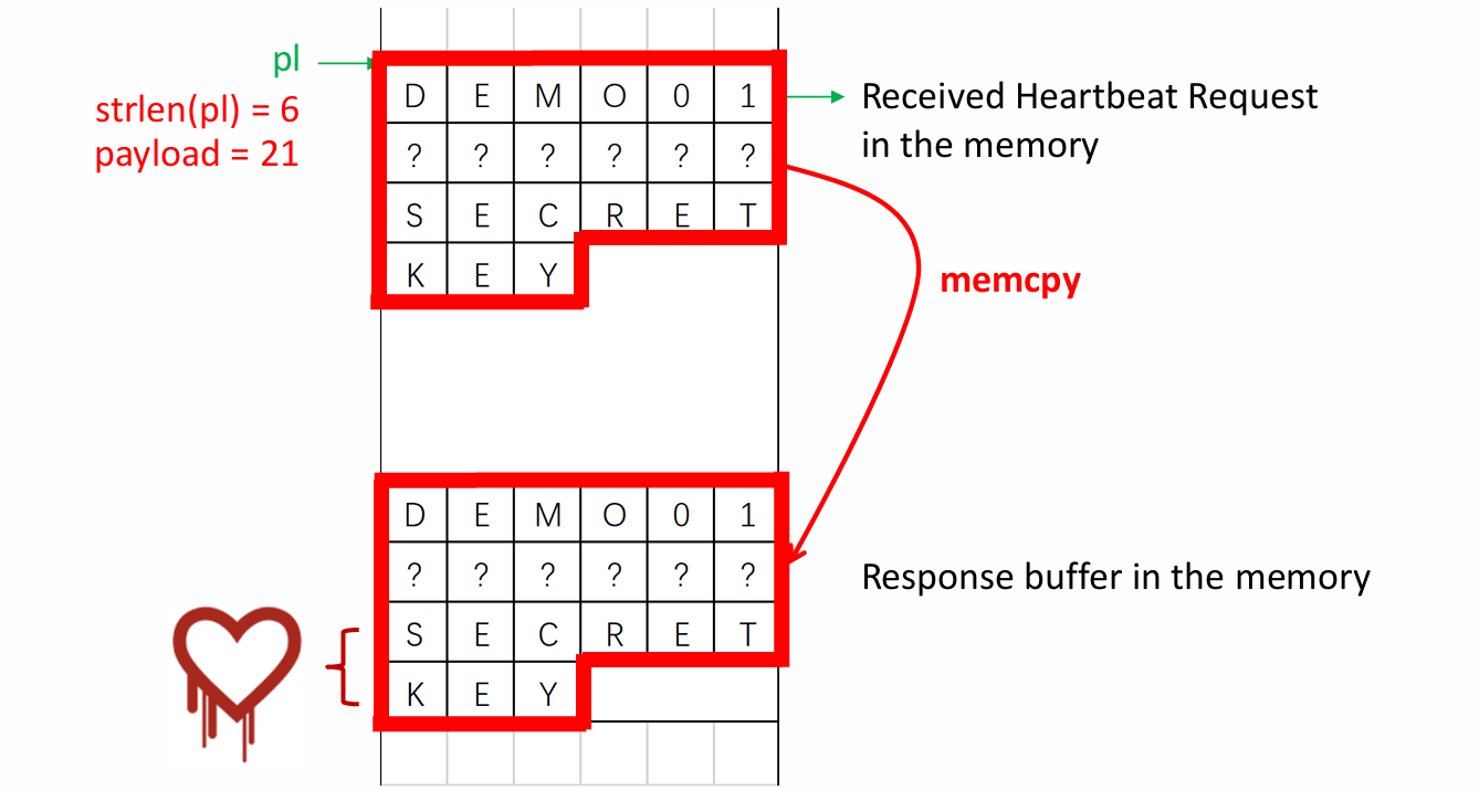
r = ssl3_write_bytes(s, TLS1_RT_HEARTBEAT, buffer, 3 + payload + padding);

The three most important variables here are pl, payload, and bp. The variable pl is a pointer to the payload string in the heartbeat request that will be copied into the response. Although the variable payload is confusingly named, it is not a pointer to the payload string, but rather an unsigned integer representing the length of the payload string. The variables pl and payload are both taken from the heartbeat request message, so they are under the control of the attacker in a heartbleed attack. The variable bp is a pointer to the response buffer where the payload string will be copied to.

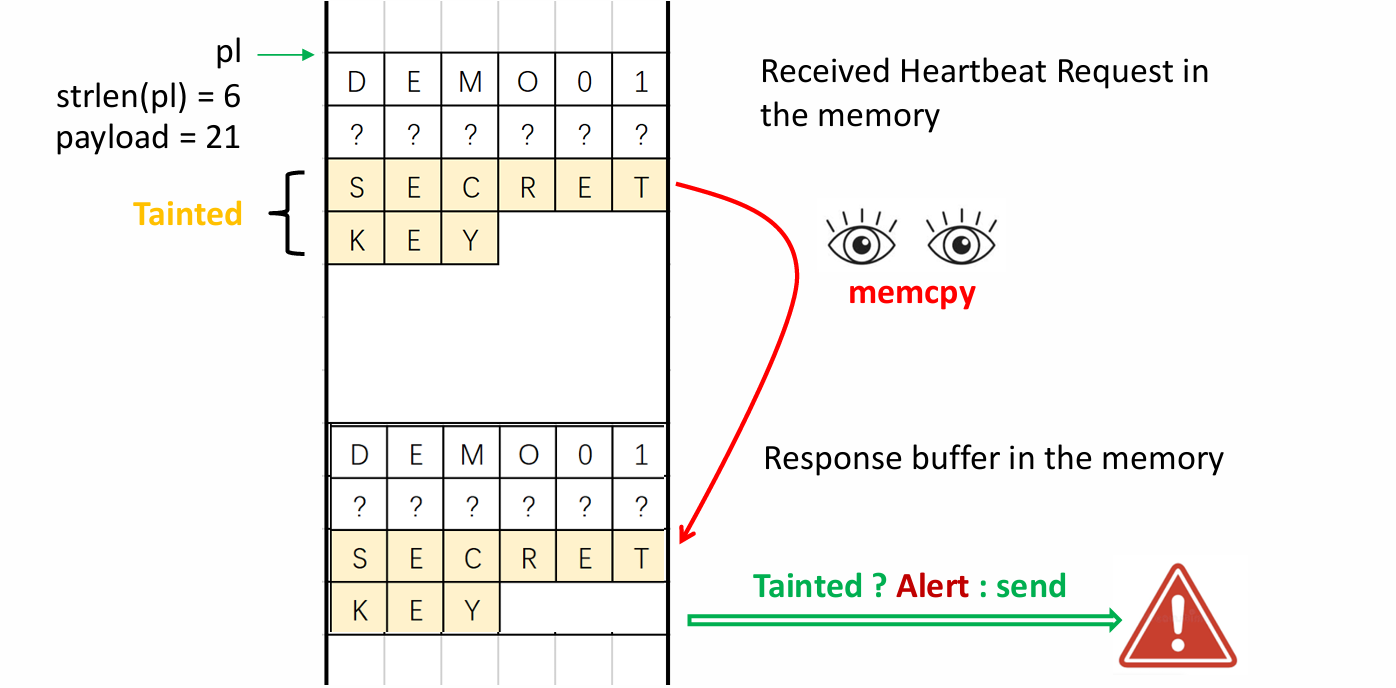
Here we will skip the prior process, which I believe is easy to understand, and move directly to the core section where the heartbleed vulnerability occurs. In line 16, the memcpy function copies the payload bytes from the pl pointer to the response buffer. As long as the attacker provides a short string for pl and a larger value for payload, the memcpy function can be tricked into copying past the request string, thus leaking any memory data immediately adjacent to the request string. In this way, the attacker can leak up to 64KB of data. Finally, the program adds some random padding bytes to the end of the response and sends the response containing the leaked information to the attacker over the network.

The following picture gives a more illustrative description of the mechanism for triggering the heartbleed vulnerability.

2.2 Define Taint Analysis

Taint analysis comprises three steps:

1. Define taint source: The taint source is the location of the program where the data you choose to trace is located. A system call, function entry point, or single instruction can be a taint source, as described in the following section.
2. Define taint sink: The taint sink is the program location where inspections are performed to determine if the location is affected by tainted data, e.g., security-sensitive operations generated (violates data integrity), or secret data leakage (violates data confidentiality).
3. Taint propagation analysis: Analyzes whether data introduced by a taint source in a program can be propagated directly to the taint sink without sanitization. The taint propagation approach defines the taint relationship between the input and the output.

---

Exercise:

1. What should be set as taint sink?
2. How does the taint data be propagated?

Solutions:

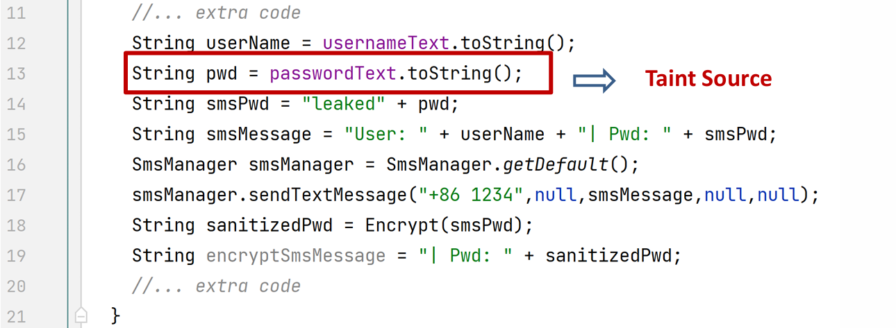
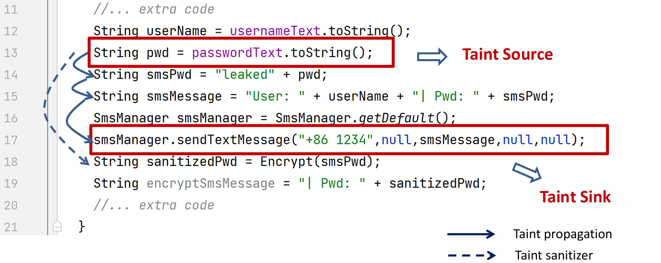
In line 13, the password is obtained from the user input passwordText, converted into a string, and assigned to the variable pwd. Since the user input may contain secret information, we define this line of code as the taint source. Later on, pwd is propagated to smsPwd and then smsMessage. Finally, in line 17, it is sent to somewhere unknown, which gives rise to the possibility of secret data leakage. Thus, we define the code in line 17 as a taint sink.

Note that in line 18, smsPwd is encrypted and assigned to sanitizedPwd. The Encrypt function can be considered as a taint sanitizer that attempts to eliminate or reduce the effect of tainted data, though it is quite limited.

2.3 Taint Analysis Approaches

2.3.1 The General Process

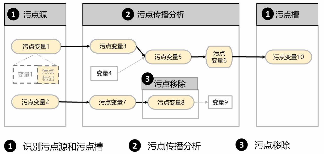
The general process of taint analysis can be mainly split into three steps as shown in the following graph:

1. Identify taint source and sink
2. Taint Propagation Analysis
3. Taint Delete

---

Step 1: Identify Taint Source and Sink

This is an important and fundamental step for taint analysis. However, due to the heterogeneity of different system models, programming languages and taint objectives, there is no general technique to specifically determine them. In practice, we usually do this manually or by some automatic taint tools. Here we present three feasible methods:

• Heuristic strategies: Collectively labeling data from inputs external to the program as taint and conservatively assuming that it may contain malicious attack data.
• Manual labeling of sources and sinks based on the APIs called by specific applications or important data types.
• Automated identification and labeling of taint sources and sinks using statistical or machine learning techniques.

---

Step 2: Taint Propagation Analysis

There are four taint analysis approaches:

• Static Explicit Taint Propagation Analysis

• Dynamic Explicit Taint Propagation Analysis

• Static Implicit Taint Propagation Analysis

• Dynamic Implicit Taint Propagation Analysis

The first two approaches are based on data flow, and the last two are based on control flow. The focus of this lesson is Dynamic Explicit Taint Propagation Analysis.

2.3.2 Static Explicit Taint Propagation Analysis

Static explicit taint propagation analysis aims to analyze the dependency between the variables in the program to check whether the data can be propagated from the taint source to the taint sink without executing and modifying the code. It primarily operates on source code or IR, relying on the techniques that convert static explicit taint propagation analysis into static data dependency analysis, e.g.:

1. Call graph
2. Analyzes specific data flow propagation within or between functions according to different program properties: propagation by direct assignment, propagation by function (procedure) calls, propagation by aliases (pointers).

Let’s look at the following snippet of Java code:

void demoMethod() {
    Dataclass a = new DataClass();
    int b = source();	// taint source
    int c = b + 10;
    foo(a,a,c)
}
void foo(DataClass x, DataClass y, int z){
    x.a1 = z;
    sink(y.a1);		// leaked!
}

In the function demoMethod, an object a is first defined. Then, the integer b is assigned the return value of the function source, making b tainted data. The value of b is later propagated to the variable c, making c also tainted. In line 5, the function foo is called with parameters a, a, and c. In foo, the first line assigns the tainted data z to x.a1, making x tainted. Afterwards, y.a1 is leaked through the sink function. Since y is not tainted, it might seem that no tainted data is leaked. However, this is not the case.

Note that in Java, parameters are passed by reference, so x and y are actually references to the same object a. So the code in line 8 not only affects x, but also affects a and z, causing the tainted data z to propagate to both x and y. Therefore, the tainted data is eventually leaked, violating the confidentiality policy.

Another question is: if the code is written in C/C++, is the tainted data still leaked? Unlike Java, C/C++ uses value passing, meaning parameters are copies of the arguments so that changes to parameters do not affect the original arguments, which prevents the propagation of tainted data. Thus, the answer is no.

2.3.3 Dynamic Explicit Taint Propagation Analysis

Dynamic explicit taint propagation analysis checks whether the tainted data can be propagated from the taint sources to the taint sinks by monitoring the execution of the program in real time, e.g., replay attacks. Dynamic explicit taint propagation analysis mainly analyzes binary instructions with the following mainstream techniques:

1. Attaches a tainted tag to the tainted data and stores it in a memory unit (RAM, registers, cache…)
2. Designs corresponding propagation logic according to the type and operands of the instructions, and analyzes the course of propagation by following the execution path

One important application of Dynamic Taint Analysis (DTA) is to solve the heartbleed vulnerability. When heartbleed vulnerability is triggered, tainted data is copied to the response buffer in the memory by memcpy. Then DTA checks if the copy contains tainted data, to decide whether the data should be allowed to be sent or not. By employing DTA, we can effectively detect and prevent heartbleed vulnerability.

---

In the heartbleed vulnerability example, the design of DTA is rather simple. We just need to define a propagation policy (which is not complicated) and the taint itself is straightforward (each byte is tagged as tainted or untainted). But with respect of more complex DTA systems, there are several factors that need to be considered, such as taint granularity, taint color and taint propagation policy.

Taint granularity is the unit of information by which the DTA system tracks taints. For example, systems with bit granularity track whether every 1 bit in a register or memory is marked as tainted, whereas systems with byte granularity track only tainted information per byte. Similarly, in a word-grained system, it tracks taint information for each word in memory, and so on.

Sometimes, we not only want to know if a value is tagged as tainted, i.e., its tainted state, but also want to know where the taint originated. In such cases, we can assign each taint a unique color and track their respective propagation paths. That’s what taint colors are meant to do. However, using taint colors requires additional memory because we need to store information about the taint colors.

Take a byte-grained DTA system as an example. It only needs to consider whether a byte is tagged as tainted or not, so it only requires one additional bit to store a tag for each byte. What about colors? If we use a byte to store colors, we would have at most 255 colors available. However, this is not practical because it would prevent us from determining whether a variable is affected by multiple taint sources.

The solution is to use only 8 different colors represented by 0x01, 0x02, 0x04, 0x08, 0x10, 0x20, 0x40, and 0x80. This allows us to easily differentiate taint sources through bitwise OR operations. For instance, we designate red as 0x01, blue as 0x02, and then the combination of them, purple, is 0x03.

A propagation policy describes how taint markings should be propagated during execution, and how to merge taint colors when multiple taint flows converge. The following table shows several examples of a propagation policy describing how taints propagate in different operations.

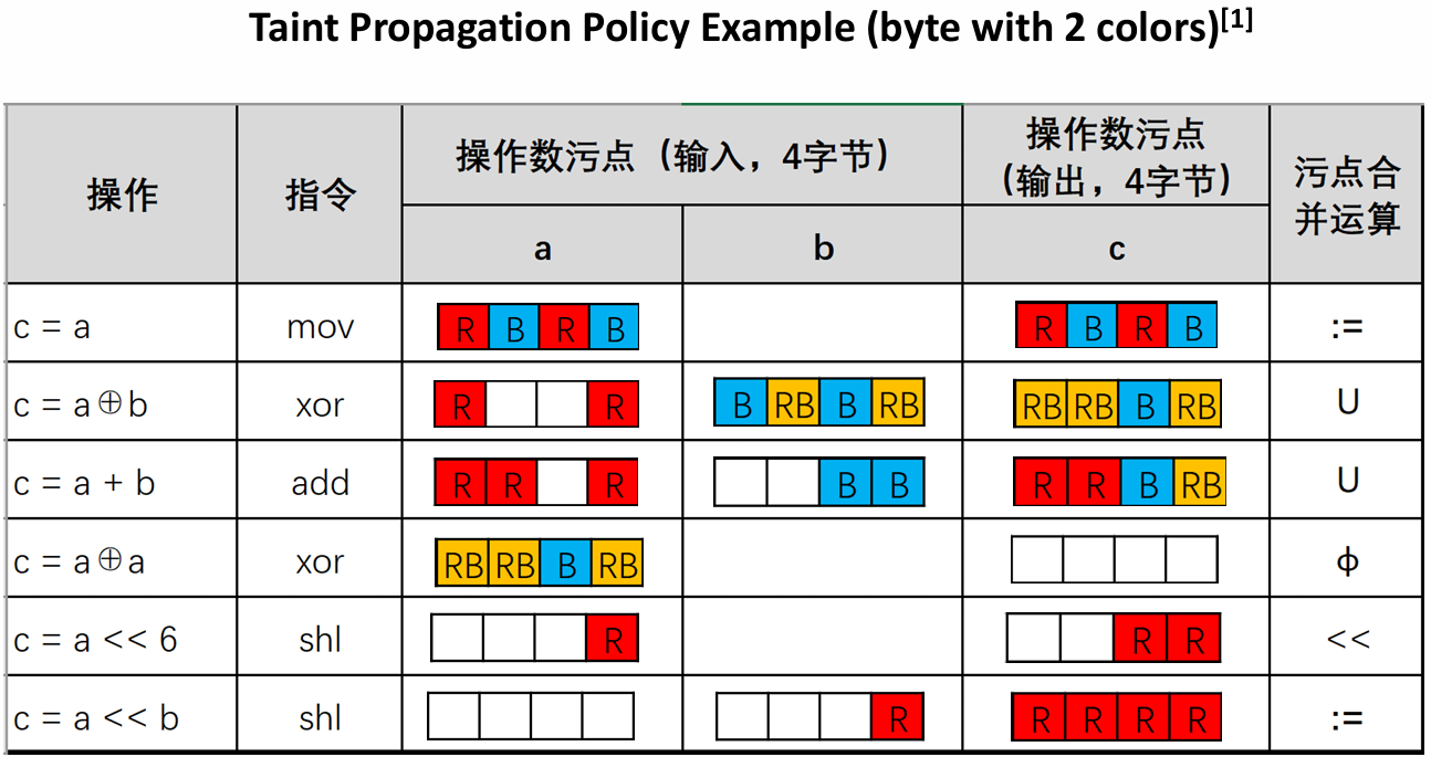
I’m not going to get into specifics on every example here, so I’ll just pick a few typical ones to talk about. Please understand the rest on your own.

The first one is a simple assignment operation, so the propagation policy is also simple. Since the output c is just a copy of a, the tainted information for c is a copy of the tainted information for a. In other words, the taint merge operator in this case is :=, an assignment operator.

The second example is the xor operation. In this case, since the output operand depends on both input operands, it does not make sense to assign the taint of only one of the input operands to the output operand. Instead, a common tainting strategy is to take the byte concatenation ($\cup$) of the taints of the input operands. For example, the highest valid byte of the first operand is labeled red (R), while the corresponding byte of the second operand is labeled blue (B). Therefore, the highest valid bit bytes of the output are labeled as their concatenation, i.e., red-blue (RB).

In the fifth example, since the second operand is a constant, the attacker cannot control all the output bytes even if he controls the input a. A reasonable strategy is to propagate the input taint only to the bytes in the output that are covered by the tainted input bytes (partially or completely), i.e., “move the taint to the left”. In this example, the attacker controls only the low byte of a and it is shifted 6 bits to the left, which means that the taint of the low byte is propagated to the two low bytes of the output.

The value of the shift (a) and the amount of the shift (b) in Example 6 are both variables. An attacker controlling b (as is the case in the example) can affect all output bytes. Therefore, the taint of b is assigned to each output byte.

2.3.4 Implicit Taint Analysis

As we have learned before, control structures implicitly affect data flow. Therefore, implicit taint analysis analyzes how tainted data propagates through the so-called implicit flow. See the following program:

void demoImplicitTaint(int a) {	// taint source
    int x, y;
    if (a > 10)	// a implicitly controls x
        x = 1;
    else
        x = 2;
    y = 10;
    System.out.println(x);	// leaked!
    System.out.println(y);
}

In this program, int a is the taint source. Although there is no program point where a is assigned to any variables, we can find that a implicitly controls x through the conditional branching in line 3. Thus, x is tainted and is leaked in line 8.

Here we present the key idea of the implicit taint propagation policy: Given a conditional branch statement $b_{r}$, which determines whether the statement $s_{t}$ will be executed or not. If the value that affects the result of $b_{r}$ also have a bearing on the value that $s_{t}$ modifies, the taint markings associated with the source operands in $b_{r}$ must be combined and associated with the destination operands in $s_{t}$.

An implicit taint analysis approach is Postdominator Tree:

• Given two nodes $m$ and $n$ in a CFG, $n$ postdominates $m$, denoted as $n\ \mathrm{pdom}\ m$ or $\mathrm{pdom}(m)=n$ iff all directed paths from $m$ to exit contain $n$.
• Given two nodes $m$ and $n$ in a CFG, $n$ immediately postdominates $m$, denoted as $n\ \mathrm{ipdom}\ m$ or $\mathrm{ipdom}(m)=n$ iff $n\ \mathrm{pdom}\ m$ and there is no node $o$ such that $n\ \mathrm{pdom}\ o$ and $o\ \mathrm{pdom}\ m$.
• A pdom tree for a CFG is a rooted tree such that
  1. it has the same set of nodes as the CFG
  2. its root is the exit node
  3. each node immediately postdominates its direct descendents in the tree
• Given two nodes $m$ and $n$ in a CFG, $n$ is control dependent on $m$ iff
  1. There is a path $P$ from $m$ to $n$ with any node $o$ in $P$ (excluding $m$ and $n$) postdominated by $n$
  2. $m$ is not postdominated by $n$
• Control flow Based Taint Propagation
  • When the execution reaches a conditional branching statement $b_{r}$, computes a set taint that contains the combination of the taint markings for $b_{r}$‘s source operands and add a pair $\langle b_{r},\{ta\}\rangle$ ($\{ta\}$ is a tainted tag) to a set $S$.
  • When the execution reaches $\mathrm{ipdom}(b_{r})$, where $b_{r}$ is a conditional branching statements, it removes from $S$ all pairs $\langle x,y\rangle$ such that $x$ is equal to $b_{r}$.
  • When a statement $s_{t}$ is executed and $S$ is not empty, it adds, for each pair $\langle x,y\rangle$ in $S$, the taint markings in $y$ to the set of taint markings to be combined and associated to $s_{t}$‘s destination operands.

---

Example:

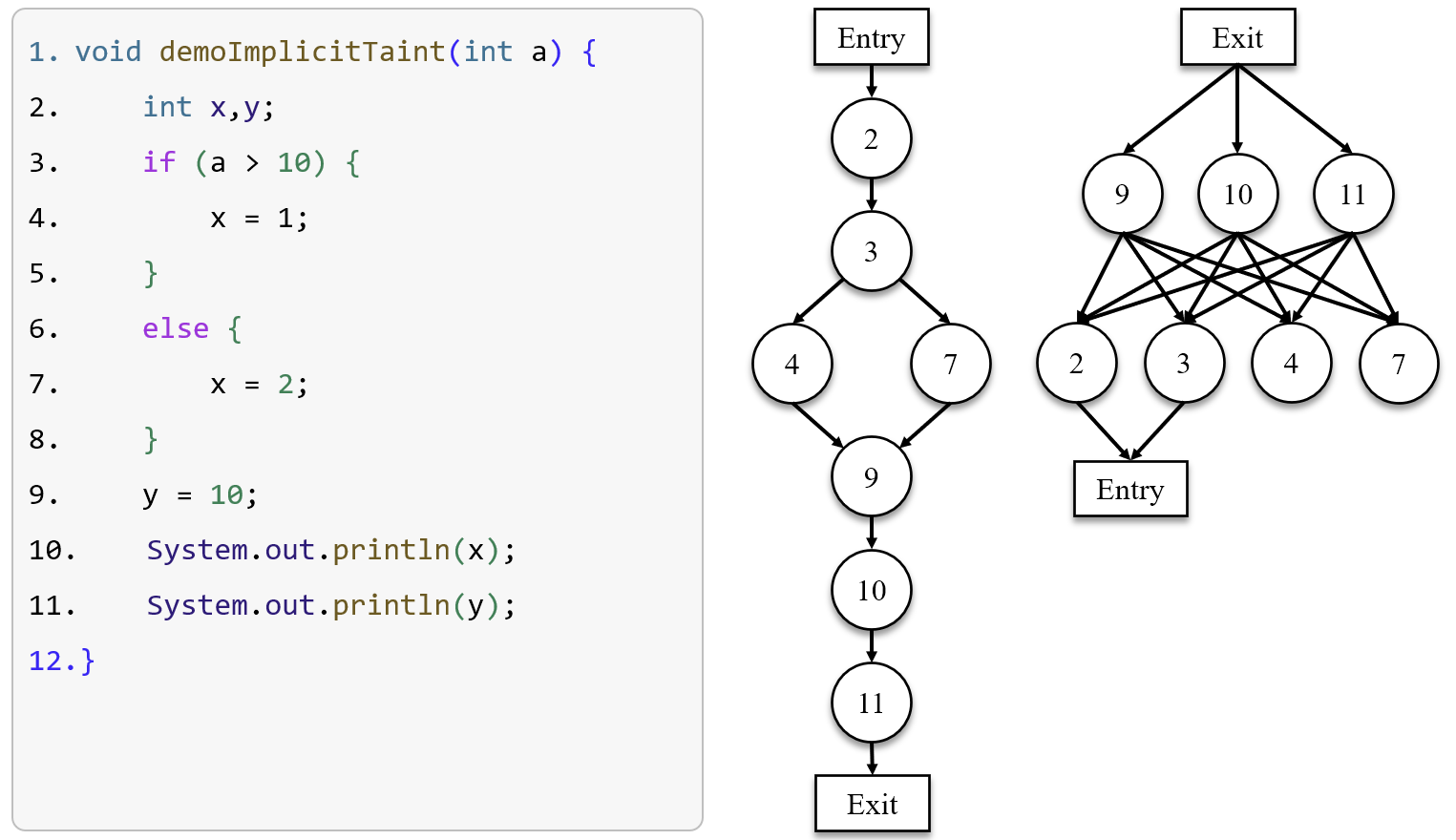
The image shows a program along with its control flow graph (mid) and postdominator tree (right). I’ll focus mainly on the process of implicit taint propagation, as the CFG and postdominator tree should be straightforward to understand. The only thing you should note is that the postdominator tree has been simplified to a rooted tree, where each node has exactly one parent node except the exit node.

Initially, $S=\emptyset$. When the conditional branch statement which contains tainted data a in line 3 is executed, we add $\langle 3,\{ta\}\rangle$ into $S$. Let’s assume that the condition is established, so it goes on to run the code in line 4, where x is implicitly tainted by the control flow. Thus, we add $\langle x,\{ta\}\rangle$ into $S$. Now, we have $S=\{\langle 3,\{ta\}\rangle,\langle x,\{ta\}\rangle\}$. Next, we are at the statement in line 9, which postdominates the statement in line 3, i.e., $\mathrm{ipdom}(3)=9$. According to the propagation rule, we are supposed to removes $\langle 3,\{ta\}\rangle$ from $S$. So now $S=\{\langle x,\{ta\}\rangle\}$. Eventually, when the execution is over, we have $S=\{\langle x,\{ta\}\rangle\}$, which means x is tainted data. Propagation ended.

In this example, we assume that a>10 is true, but what if it isn’t? Does the assumption affect the result? The answer is yes. We will talk about this in the next section.

2.4 Over-taint and Under-taint

Under-taint and over-taint problems are challenges of taint analysis.

Under-taint means that values that “should” be marked as tainted is not marked as tainted, which is often caused by taint policies.

The problem of an excessive number of tainted markers leading to a large propagation of tainted variables is known as over-taint. A way of solving the problem is that we can choose appropriate taint marking branches to propagate taints.

See the following code:

void demoOverTain() {
	int a = source();
    int x = 0, y = 0, z = 0;
    int w = a + 10;
    if (a == 10) {
		x = 1;
    } else if (a > 10 && w <= 23) {
    	y = 2;
    } else if (a < 10) {
    	z = 3;
    }
    sink(x, y, z);
}

As we can see, there are three conditional branches in the program. The major difference between them is their scopes of information leaked. Once the first condition a == 10 is established, i.e., x becomes 1, attackers can easily obtain the true value of the tainted data 10, so this branch is rather dangerous. The second considition a > 10 && w <= 23 can only be true when a is 11, 12, or 13. Attackers have a one-third chance of guessing the correct value of a when this condition is true. In contrast, the third branch is least dangerous, because it covers a wide range of the possible values of a. In conclusion, given the priority of the three branches, we should put more focus on the first one. So a plausible option is to choose the first branch to propagate taints in this case.

2.5 Shadow Memory

So far, I’ve shown that the taint tracker can track the taint for each register or byte of memory, but haven’t described where the taint information is stored. To store information such as register or memory taint location and taint color, the DTA engine maintains dedicated Shadow Memory. Shadow memory is a virtual memory area allocated by the DTA system to track the taint status of the rest of the memory. Typically, the DTA system also allocates a special structure in memory for tracking CPU register taint information.

The structure of the shadow memory depends on the taint granularity and the number of supported taint colors. The following figure shows the distribution of shadow memory for tracking up to 1 or 8 colors at byte granularity, respectively.

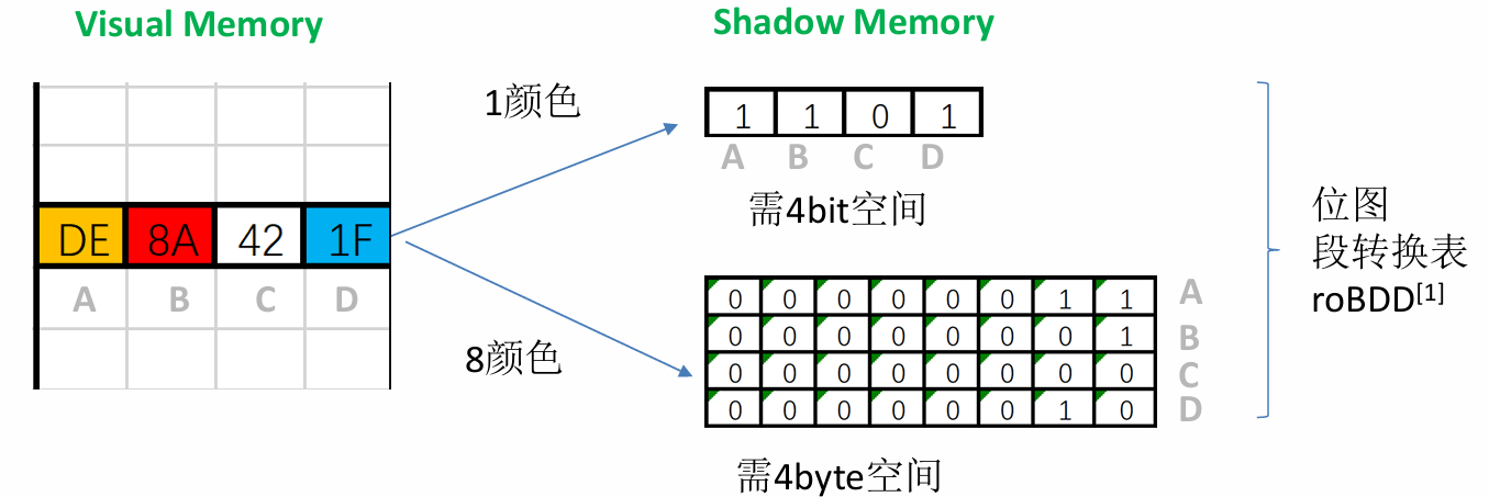
This type of shadow memory is called bitmap-based shadow memory. It stores 1 bit of taint information for each byte of virtual memory, so it can only represent one color, i.e., whether or not each byte of memory is marked as tainted.

2.6 The DyTAN Framework

DyTAN (Dynamic Taint Analysis Framework) is a generic dynamic taint analysis framework that provides a high degree of flexibility and customizability, supports both data-flow and control-flow taint analysis, and does not depend on a custom runtime system. The framework allows users to customize all aspects of taint analysis as needed, such as taint sources, propagation strategies, and taint sinks.

The following graph illustrates the architecture of the DyTAN framework:

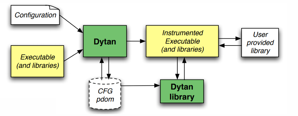
The DyTAN framework generates control flow graphs and postdominator trees by reading configuration files, instrumenting executables and libraries, and generating instrumented programs and libraries. The instrumented program calls functions in the DyTAN libraries at runtime to track the source and flow of data, and passes the results to user-provided libraries for further processing. This architecture makes DyTAN highly flexible and customizable for different dynamic taint analysis scenarios.

Footnotes

1. Data is considered low-integrity such that it is unreliable or unauthenticated, e.g., user input. ↩

2. There is a formal discrepancy between the definitions given by Prof. Dr. Michael Pradel at USTUTT and those presented in ECNU’s slides. However, it should not be a major issue for students who have learned discrete math. Just understand $SC$ equals $s$, $\preceq$ equals $\rightarrow$, other elements are omitted and move on. ↩